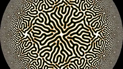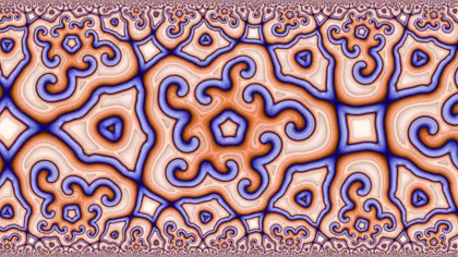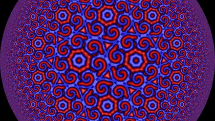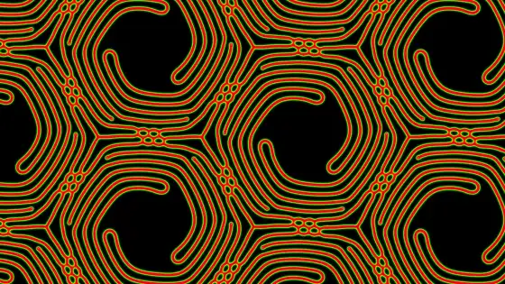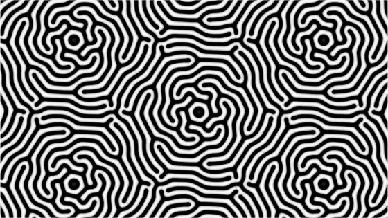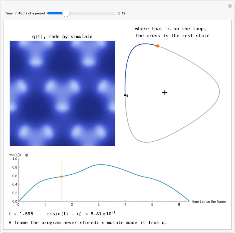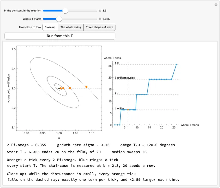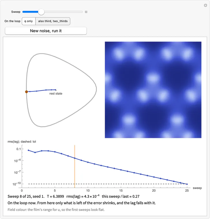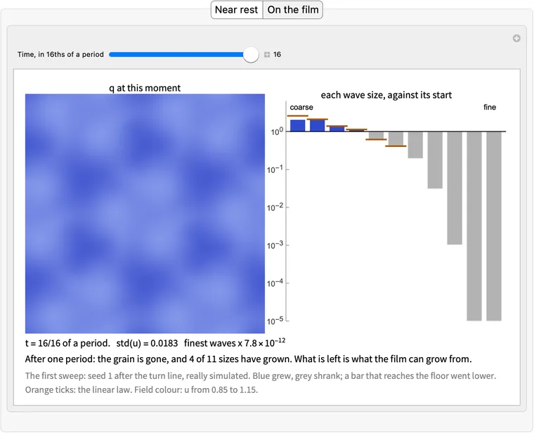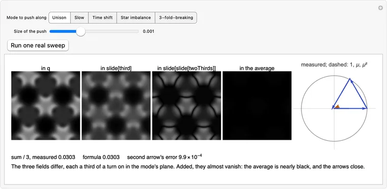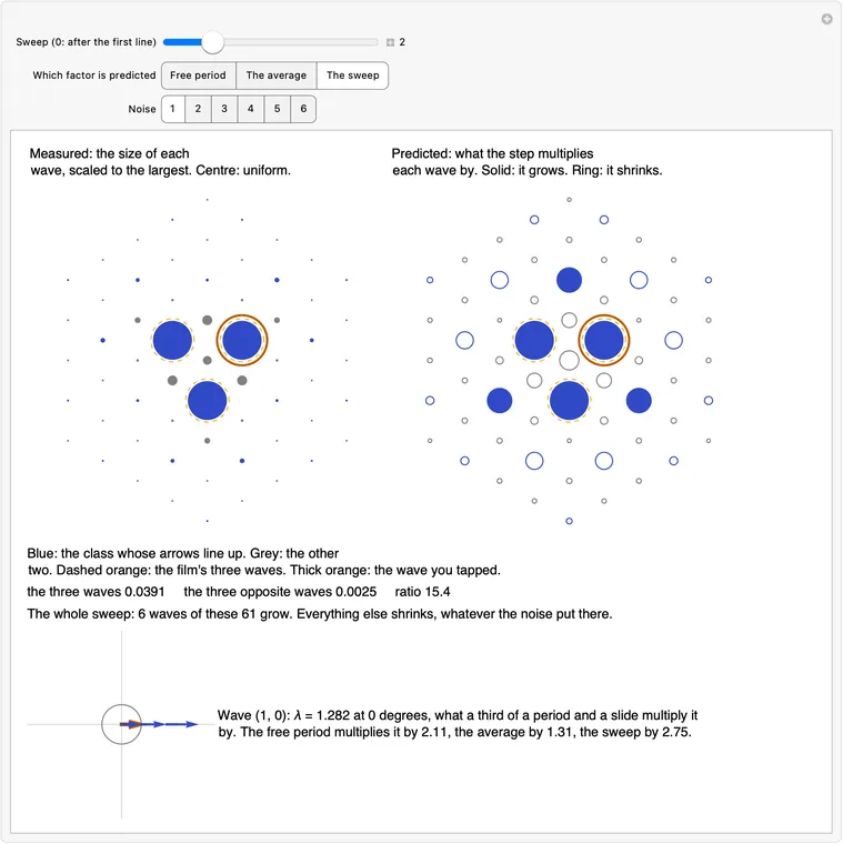
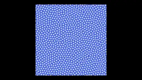
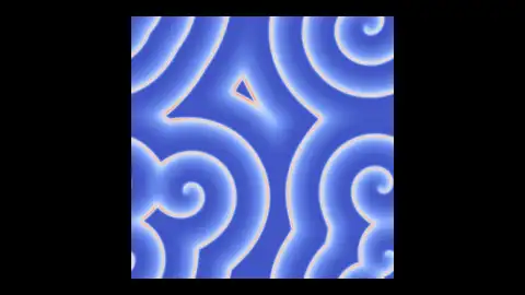
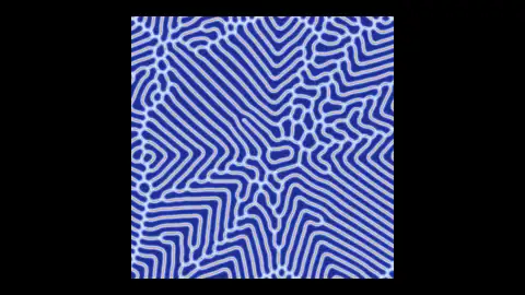
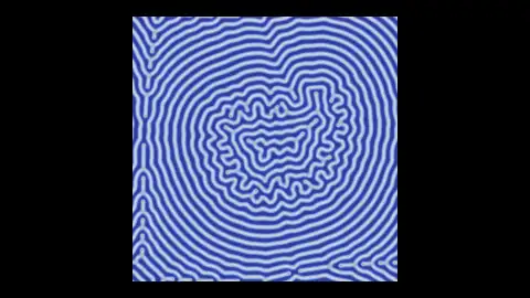
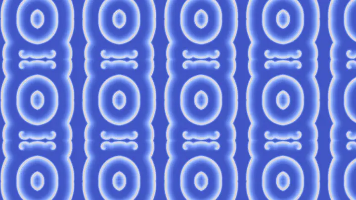
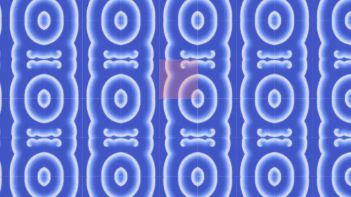
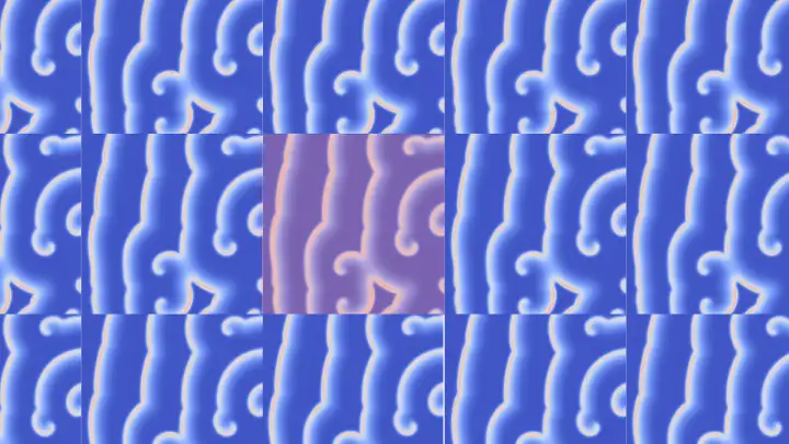
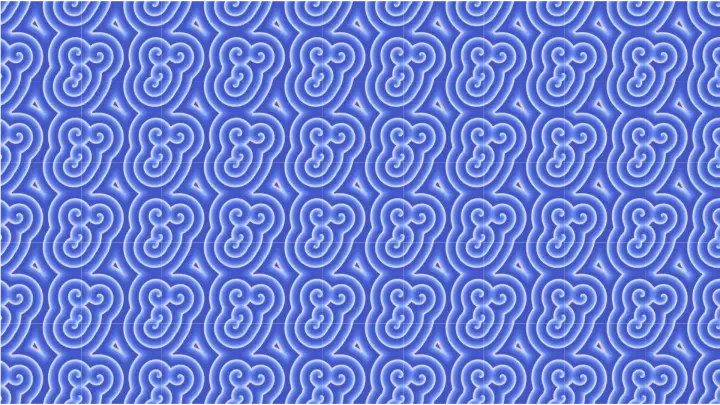
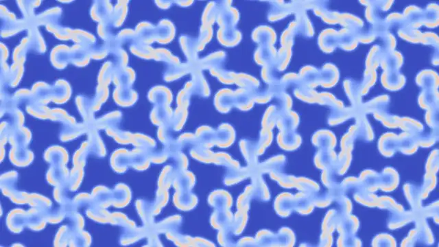
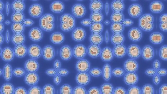
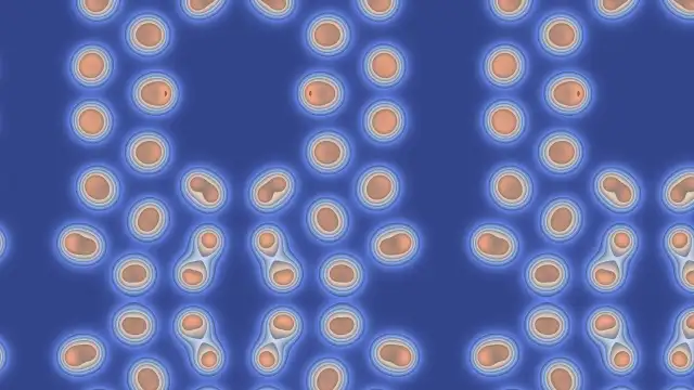
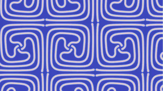
Symmetric animation - simplified

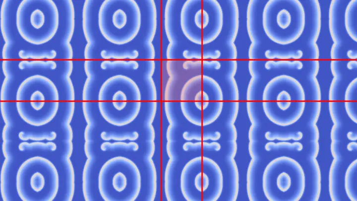
Can Vladimir Bulatov's SymSim (Symmetric Simulation) run on a ? Yes. Give each side of the a time delay, and read the that fraction of a period ago. From noise it forms the published Brusselator film: 12 of 12 seeds in an independent simulator, 9 of 9 in his own WebGL engine.

Part 1

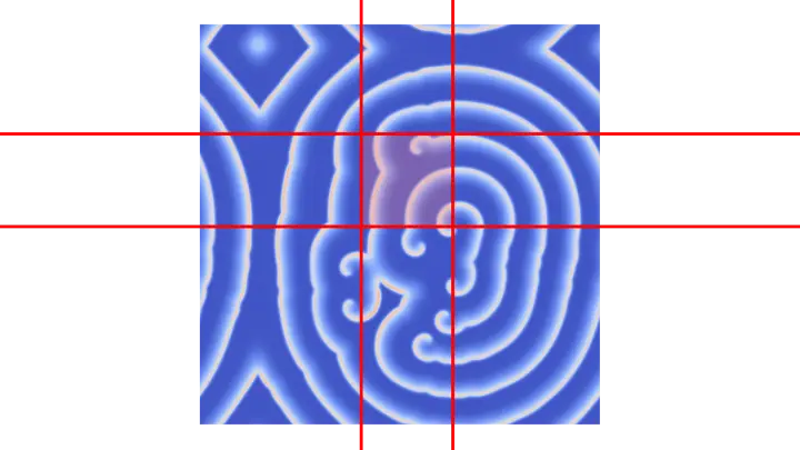
How SymSim makes a simulation symmetric. He keeps the equation and the simulation grid and adds one step: copy every cell outside a small tile from its matching point inside the tile, then simulate on. The seams, the jumps where the tile's copies meet, heal by themselves.

Vladimir Bulatov, JMM 2025 slide 2: His summary (JMM = Joint Mathematics Meeting)
His summary (JMM = Joint Mathematics Meeting) JMM 2025, slide 2

1. The goal: patterns both natural and symmetric

"Our goal is to create process for generation of natural animated symmetric patterns"JMM 2025, slide 2

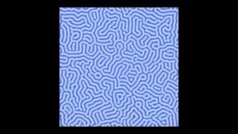
Patterns from physical laws are rarely symmetric. He takes one such law, the Gray-Scott equation: two chemicals that react and diffuse.

, and are the concentrations of chemicals and . The reaction makes more , and slowly turns inert. A simulation solves this on a grid of cells: each step updates a cell from itself and its neighbours. Two numbers, , pick the regime: the kind of pattern.

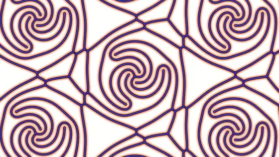
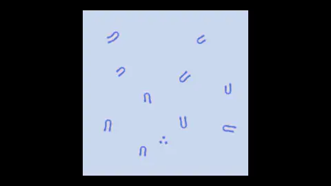
Vladimir Bulatov, JMM 2024 slide 9: Mazes
Mazes JMM 2024, slide 9
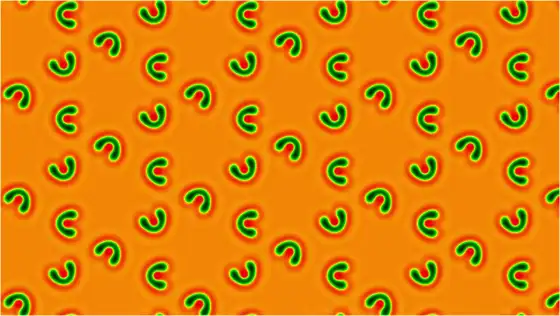
Vladimir Bulatov, JMM 2024 slide 10: Static spots
Static spots JMM 2024, slide 10
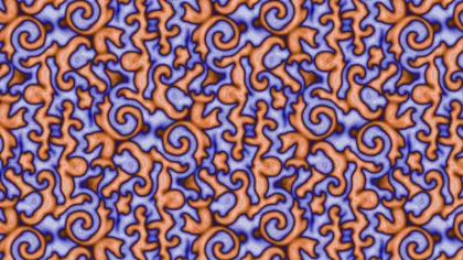
Vladimir Bulatov, JMM 2024 slide 18: Spiral waves
Spiral waves JMM 2024, slide 18

Try it: his named regimes

= = steps 0

Colour shows . Tap to add . No symmetry yet.

More regimes, and the numbers behind this demo
Vladimir Bulatov, JMM 2024 slide 4: Unstable loops
Unstable loops JMM 2024, slide 4
Vladimir Bulatov, JMM 2024 slide 6: Parallel waves
Parallel waves JMM 2024, slide 6
Vladimir Bulatov, JMM 2024 slide 14: U-skate gliders
U-skate gliders JMM 2024, slide 14

128 by 128 cells with wrap-around, explicit Euler with time step , , , his nine-point Laplacian with edge weight 0.8 and corner weight 0.2. Names and , values are from his preset table (gray_scott_presets.js). Greek letters in his preset names, as in "Worms (mu)", are Pearson's pattern classes. His slides write the Laplacian as , and the second equation as : a typo for (JMM 2024, slide 2). His U-skate needs a hand-placed seed, so it is left out of the live list.

2. The obvious try: Simple Symmetrization

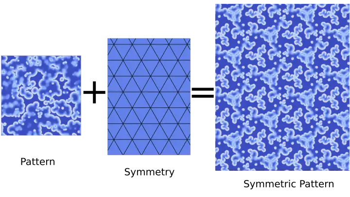
Take a finished pattern and copy it around. Pick one of the 17 , build its (the tile), place the pattern inside, and fill the plane by .

Vladimir Bulatov, JMM 2024 slide 21: Build the domain
Build the domain JMM 2024, slide 21
Vladimir Bulatov, JMM 2024 slide 22: Place the pattern
Place the pattern JMM 2024, slide 22
Vladimir Bulatov, JMM 2024 slide 24: Reverse pixel mapping
Reverse pixel mapping JMM 2024, slide 24
Vladimir Bulatov, JMM 2024 slide 25: Perfectly symmetrical
"Perfectly symmetrical" JMM 2024, slide 25

Try it: pick a , look for jumps along the white lines

Value jump at the domain's sides:

    Tap a point: the white path is the moves that bring it home to the outlined domain.

    4 of 17"Simple Symmetrization works only for 4 out of 17 wallpaper groups": the four made of mirrors only, *2222, *442, *632 and *333. (JMM 2024, slide 44) On the other 13 the copies do not match: a jump along the domain's sides, a seam.
    Vladimir Bulatov, JMM 2024 slide 54: *2222: Pattern matches along the fundamental domain sides
    *2222: "Pattern matches along the fundamental domain sides" JMM 2024, slide 54
    Vladimir Bulatov, JMM 2024 slide 59: O: No match along sides
    O: "No match along sides" JMM 2024, slide 59
    About this demo and his test slides

    The pattern is one finished Fingerprints run (, , 128 by 128). His own test image, (JMM 2024, slide 26), is a spiral. His slide 29 is titled *442, but its image is the *632 test, so it is filed here under *632. Domain sizes are ours, chosen so each domain fits inside the grid.

    3. "Where from comes the magic?"

    Back to group o, but now the tile is the whole simulation grid. There is no seam at all:

    Vladimir Bulatov, JMM 2024 slide 71: Pattern magically seamlessly matches
    "Pattern magically seamlessly matches" JMM 2024, slide 71

    The reason is periodic boundary conditions (PBC), or wrap-around: a cell on the grid's edge takes its missing neighbours from the .

    "Using PBC is equivalent to a simulation on the wallpaper group (O) - topological "JMM 2024, slide 72

    Try it: "Boundary" has no effect on the pattern (JMM 2024, slide 73)

    Jump across the wrap edge stdacross a line inside std

    Each arrow: a cell past one edge reads the far edge. Tap a cell: its copies light up.

    The simulation saw its own gluing while it ran, so the seam was never there. His question:

    "Can we apply PBC idea to other symmetries?"JMM 2024, slide 85

    4. The orbifold, in plain words

    Glue together every pair of points the group calls the same. What is left is a small closed surface: the orbifold. A symmetric pattern on the plane is an ordinary pattern on that surface. The equation allows this: it has no preferred place or direction, so a moved or mirrored solution is still a solution.

    "An orbifold can be cut and flattened. The flattened orbifold will tile the whole space. If the pattern is seamless on the orbifold the tiled pattern will be seamless as well."Gathering 4 Gardner (G4G) paper, page 2

    Cut and flattened, it is the fundamental domain plus a rule for which side glues to which. What each rule does to a cell's at a side:

    Mirror

    Glued to itself. A neighbour across reads its own reflection, so the value cannot jump. The slope can.

    Rotation

    Glued to the next side, turned. Around a neighbours wrap: by on 333.

    Glide

    Glued to the far side, flipped.

    Translation

    Glued to the far side, as is. This is PBC.

    Filled dots: the stencil. Open: its neighbours outside the domain. Arrow: where each reads. Thick: the sides glued.

    So a mirror side reads back the value beside it, while any other side reads a far place holding an unrelated value, since the simulation never coupled the two. Hence 4 of 17: the four groups whose sides are all mirrors.

    Which groups have which sides
    SidesGroups
    All mirrors (4): his "good" list*2222, *442, *333, *632
    Some mirrors (6): a jump only on the others4*2, 3*3, 2*22, 22*, **, *x
    No mirrors (7)442, 632, 333, 2222, 22x, xx, o

    Read from his side lists in WallpaperGroups.js: a side's word (the reflections that glue it) of one reflection is a mirror; two crossing mirrors a rotation; two parallel mirrors a translation; three a glide. For the whole notation, see Two Dollars of Symmetry.

    5. The main idea: symmetrize, then simulate

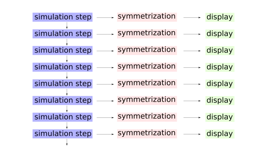
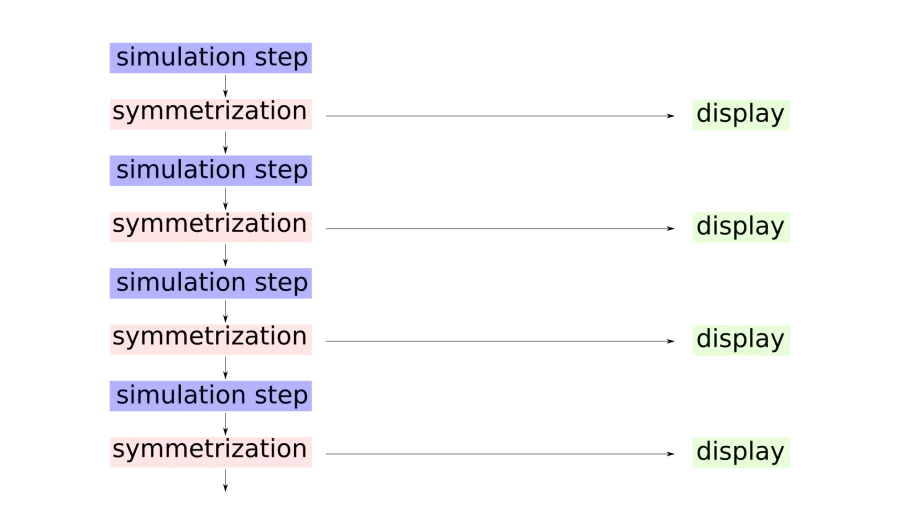
    "We replace simulation step with a pair - (symmetrization + simulation)"JMM 2024, slide 86

    The open dots of section 4 need somewhere to live, so take a plain grid larger than the domain; the cells outside it are . Write the field as . Symmetrizing, , overwrites every ghost with its value inside the domain, by the reverse pixel mapping of section 2, here called :

    Let be simulation steps on the whole grid. Against Simple Symmetrization, the only change is the inside:

    Both display ; only SymSim feeds it back. Now a cell beside a side reads its glued neighbours through the ghosts, as a cell at the grid's edge does under PBC. The simulation sees the gluing, and diffusion smooths the jump away.

    Vladimir Bulatov, JMM 2025 slide 31: Simple: display only
    Simple: display only JMM 2025, slide 31
    Vladimir Bulatov, JMM 2025 slide 32: SymSim: fed back
    SymSim: "fed back" JMM 2025, slide 32

    Try it: watch the seams heal

    stdsteps 0

    The grid, simulated

    The plane, tiled

    Step by hand

    Move to "once, then never" and press Restart. On xx the seams stay away: this is a matching grid, its wrap-around already one of the group's moves, so a symmetric field stays symmetric. No square grid can match 333: wrap-around error creeps in from the edge, and symmetrizing holds it off.

    His own run, on xx

    How large can be

    Between symmetrizations the whole grid evolves. If the ghosts hold the true continuation, the domain's stencils read what they would read on the infinite plane, until the error from the grid's own wrong wrap-around arrives. So the error must not cross the :

    Across his 65 saved wallpaper presets the grid is 1.7 to 20 times wider than the domain (symsim-presets.json).

    His code against his talks
    • The interval. The talks say once per 1000 steps. The code symmetrizes once per frame, every stepsCount steps (this page's ): Gray-Scott median 181, median 10.
    • symMix blends ghosts only, since cells inside the domain map to themselves. It is not an average over the group. All 165 presets set it to 1.
    • Interpolation. A ghost's home falls between grid points. The talk says "linear or quadratic" (JMM 2025, slide 26); his symmetrization is linear only.
    • Few lookups. His presets stop after symIterations = 1 to 10 moves, so far ghosts stop on another ghost. The cells a stencil reads almost all arrive.
    • The stencil. Weights 0.8 and 0.2 give 1.2 times the isotropic Laplacian. That is what lets a square grid carry and symmetry.

    Read from his code at GitHub main 1fbb615; the preset counts are in symsim-presets.json.

    More of his runs
    333, no SymSim: "Persistent discontinuities" JMM 2025, slide 33
    333, SymSim: "Discontinuities are instantly disappearing" JMM 2025, slide 34
    "Simulation is effectively performed on a 2D torus" JMM 2025, slide 15
    "longer simulation completely eliminates the wrinkles" JMM 2024, slide 106
    Vladimir Bulatov, JMM 2024 slide 107: We got perfect animated pattern with symmetry (XX)
    "We got perfect animated pattern with symmetry (XX)" JMM 2024, slide 107
    Vladimir Bulatov, G4G 2024 slide 30: 442, step 0
    442, step 0 G4G 2024, slide 30
    Vladimir Bulatov, G4G 2024 slide 41: 442, step 100
    442, step 100 G4G 2024, slide 41
    Vladimir Bulatov, JMM 2024 slide 108: *2222, Simple: the mirrors show kinks
    *2222, Simple: the mirrors show kinks JMM 2024, slide 108
    Vladimir Bulatov, JMM 2024 slide 109: *2222, SymSim: the kinks are gone
    *2222, SymSim: the kinks are gone JMM 2024, slide 109
    The demo's set-up

    Fingerprints, 128 by 128, started from a running pattern, on a JavaScript copy of his code. xx has his size parameters , so the domain is a quarter of the grid and the grid's wrap-around is in the group. 333 has , and no hexagonal group can match a square grid. The first 100 steps run slowly, about 9 seconds, so the healing can be seen, then it speeds up and stops at 30,000 steps, the chart's right edge. The dashed line is the same measure across the same lines before any symmetrization.

    6. It works: the seams heal

    Measured on a tested JavaScript of his code, 256 by 256. Its limits are in the bars.

    Seams fall from 1.5 std to the no-seam level by step 100

    0.010.11010100100010,000steps since the first symmetrizationseam, stdno seam 0.09median at step 0: 1.47 stdmedian at step 1: 1.15 stdmedian at step 10: 0.40 stdmedian at step 20: 0.23 stdmedian at step 50: 0.12 stdmedian at step 100: 0.08 stdmedian at step 200: 0.06 stdmedian at step 500: 0.06 stdmedian at step 1000: 0.05 stdmedian at step 5000: 0.07 stdmedian at step 20000: 0.04 stdmedian 1.470.08
    Nine runs: 3 regimes on 333, 632 and xx. Blue: the median. The fall goes like : diffusion smoothing a jump.
    "Only 4 out of 17": true of the value, not the slope

    "works only for 4 out of 17" (JMM 2024, slide 44)

    The value jump is zero on exactly his four, but their slope still jumps

    value jumpslope jump*2222*2222: value jump 0.00 std0*2222: slope jump 1.321.32*442*442: value jump 0.00 std0*442: slope jump 1.271.27*632*632: value jump 0.00 std0*632: slope jump 1.331.33*333*333: value jump 0.00 std0*333: slope jump 1.511.512*222*22: value jump 0.73 std0.732*22: slope jump 1.301.30****: value jump 1.02 std1.02**: slope jump 1.161.1622*22*: value jump 1.08 std1.0822*: slope jump 1.181.18*x*x: value jump 1.09 std1.09*x: slope jump 1.181.184*24*2: value jump 1.17 std1.174*2: slope jump 1.091.093*33*3: value jump 1.30 std1.303*3: slope jump 1.151.1522222222: value jump 1.42 std1.422222: slope jump 0.880.88442442: value jump 1.47 std1.47442: slope jump 0.950.95333333: value jump 1.49 std1.49333: slope jump 1.051.0522x22x: value jump 1.49 std1.4922x: slope jump 0.990.99xxxx: value jump 1.52 std1.52xx: slope jump 0.950.95oo: value jump 1.53 std1.53o: slope jump 0.960.96632632: value jump 1.57 std1.57632: slope jump 1.001.00
    Value in std, slope in rms gradients. Others: value 0.73 to 1.57 std. Slope: 1.27 to 1.51 on his four, 0.88 to 1.05 on groups with no mirror side.

    His own paper says the rest: "discontinuity of derivatives along reflection lines generates obvious visible artifacts" (Gathering 4 Gardner (G4G) paper, page 2). The good groups are continuous, not smooth, which is why SymSim helps them too.

    "Once per 1000 simulation steps": true, up to a limit

    "the symmetrization step can be used only once per 1000 simulation steps" (JMM 2024, slide 121)

    At the seam stays near 0.1 std in most regimes, but fast on a small reaches 1.0

    00.51501002003005001000symmetrize every K stepsseam, stdGinzburg-Landau, xx, margin 144 px, K=50: 0.06 stdGinzburg-Landau, xx, margin 144 px, K=100: 0.06 stdGinzburg-Landau, xx, margin 144 px, K=200: 0.06 stdGinzburg-Landau, xx, margin 144 px, K=300: 0.06 stdGinzburg-Landau, xx, margin 144 px, K=500: 0.06 stdGinzburg-Landau, xx, margin 144 px, K=1000: 0.06 stdFingerprints, 333, margin 39 px, K=50: 0.09 stdFingerprints, 333, margin 39 px, K=100: 0.09 stdFingerprints, 333, margin 39 px, K=200: 0.07 stdFingerprints, 333, margin 39 px, K=300: 0.07 stdFingerprints, 333, margin 39 px, K=500: 0.09 stdFingerprints, 333, margin 39 px, K=1000: 0.09 stdSlow Ginzburg-Landau, 333, margin 39 px, K=50: 0.03 stdSlow Ginzburg-Landau, 333, margin 39 px, K=100: 0.03 stdSlow Ginzburg-Landau, 333, margin 39 px, K=200: 0.03 stdSlow Ginzburg-Landau, 333, margin 39 px, K=300: 0.03 stdSlow Ginzburg-Landau, 333, margin 39 px, K=500: 0.03 stdSlow Ginzburg-Landau, 333, margin 39 px, K=1000: 0.03 stdWaves, xx, margin 72 px, K=50: 0.10 stdWaves, xx, margin 72 px, K=100: 0.10 stdWaves, xx, margin 72 px, K=200: 0.10 stdWaves, xx, margin 72 px, K=300: 0.11 stdWaves, xx, margin 72 px, K=500: 0.09 stdWaves, xx, margin 72 px, K=1000: 0.09 stdChaos, xx, margin 72 px, K=50: 0.05 stdChaos, xx, margin 72 px, K=100: 0.05 stdChaos, xx, margin 72 px, K=200: 0.05 stdChaos, xx, margin 72 px, K=300: 0.05 stdChaos, xx, margin 72 px, K=500: 0.04 stdChaos, xx, margin 72 px, K=1000: 0.06 stdGinzburg-Landau, 333, margin 39 px, K=50: 0.07 stdGinzburg-Landau, 333, margin 39 px, K=100: 0.06 stdGinzburg-Landau, 333, margin 39 px, K=200: 0.06 stdGinzburg-Landau, 333, margin 39 px, K=300: 0.08 stdGinzburg-Landau, 333, margin 39 px, K=500: 0.13 stdGinzburg-Landau, 333, margin 39 px, K=1000: 1.00 stdGinzburg-Landau, 333, margin 79 px, K=50: 0.06 stdGinzburg-Landau, 333, margin 79 px, K=100: 0.07 stdGinzburg-Landau, 333, margin 79 px, K=200: 0.07 stdGinzburg-Landau, 333, margin 79 px, K=300: 0.08 stdGinzburg-Landau, 333, margin 79 px, K=500: 0.17 stdGinzburg-Landau, 333, margin 79 px, K=1000: 0.83 stdGinzburg-Landau, xx, margin 72 px, K=50: 0.06 stdGinzburg-Landau, xx, margin 72 px, K=100: 0.06 stdGinzburg-Landau, xx, margin 72 px, K=200: 0.06 stdGinzburg-Landau, xx, margin 72 px, K=300: 0.06 stdGinzburg-Landau, xx, margin 72 px, K=500: 0.06 stdGinzburg-Landau, xx, margin 72 px, K=1000: 0.33 stdGL, 333, 39 pxGL, 333, 79 pxGL, xx, 72 pxother regimes,GL at 144 px
    Mean seam just after a symmetrization, in std. GL: Ginzburg-Landau at his default. px: the margin. None of these grids match the group: xx here has , not the of section 5.

    On a matching grid the only limit is instability: at the worst measured rate, float32 round-off reaches 1% in about 1800 steps. On any other grid the decides. His saved wallpaper Ginzburg-Landau presets agree: they run at to , none near 1000.

    "True solutions": exact on a matching grid, a small error on others

    "true solutions of the original equations" (JMM 2024, slide 121)

    On a matching grid the tiled pattern solves to round-off; 333 on a square grid keeps a floor of 14–20%

    1e-151e-101e-51Plain periodic runPlain periodic run: 5.9e-156e-15xx, matching, K=1xx, matching, K=1: 6.3e-156e-15xx, matching, K=1000xx, matching, K=1000: 7.5e-157e-15*2222, matching, K=1*2222, matching, K=1: 6.5e-156e-15333, cubic lookup, K=1333, cubic lookup, K=1: 3.6e-20.04333, K=1000333, K=1000: 1.4e-10.14333, K=1333, K=1: 2.0e-10.20Simple, *2222Simple, *2222: 1.2e+01.17Simple, 333Simple, 333: 2.8e+02.84Simple, xxSimple, xx: 4.2e+04.16
    The residual: how far the tiled pattern is from solving his scheme, next to tile edges, as a fraction of the diffusion term. Fingerprints. A matching grid: its wrap-around is in the group. Simple: no feedback.

    Inside the domain, away from its sides, the residual is round-off. The 333 floor sits on the domain's copies and next to its sides, because they are read through , and it does not shrink with a finer grid. A cubic lookup does shrink it.

    "Very little cost": true at large

    "very little cost" (JMM 2024, slide 121)

    0.3 msone symmetrization, 128 by 128
    3.6 ms20 simulation steps, same grid

    One symmetrization costs about as much as 1.7 steps: at it nearly triples the time, at it adds 0.2%.

    "Any number of dimensions": stated, not shown

    "can be used in any number of dimensions" (Gathering 4 Gardner (G4G) paper, page 7). It appears in the paper only, and every grid in his apps is 2D. Part 2 tries it on a crystal whose third axis is time.

    Is the symmetric solution stable? Measured here

    Settled at , then symmetrization off, in double precision, with a nudge. On a matching grid the symmetric subspace is exactly invariant, so what remains is stability. On xx: fingerprints, mazes, spots and loops hold for 60,000 steps; chaos, waves and fast lose the symmetry at to per step. On 442 even fingerprints loses it, at step 30,000. On a grid that does not match, switching off is immediate: the difference passes 1% at step 1, in 20 of 20 runs. That is the grid's seam, not an instability. Source: symsim2d.json, summary.e.

    How it was measured
    • Value and slope jump: across the domain's sides of a finished plain run; 6 regimes, 3 seeds each; value in field standard deviations, slope in rms gradients (summary.a). The same measure across the same line with no seam reads 0.07 to 0.09.
    • Seam against steps: , groups 333, 632, xx, regimes fingerprints, waves and (summary.b). Between steps 1 and 100 the exponent is to . He says "original wrinkles almost gone" after 100 of his steps (JMM 2024, slide 105). His slide steps cannot be matched to these: a slide "SymSim step" is a frame of several Euler steps.
    • Every : mean seam just after a symmetrization, over the late half of a run, one seed (summary.k). Reading " below over speed" from this table is ours, not a direct speed measurement.
    • Waves and chaos at show no seam, yet on a non-matching grid the domain has moved far from the run: distance 1.3 to 1.5, against 0.001 at (summary.c). On hexagonal groups, symmetrizing less often gives smaller seams, since each symmetrization interpolates: loops on 333 read 0.45 at and 0.18 at .
    • Next to the sides of the domain: residual 0.01 on 333 at , 0.10 at ; away from them, .
    • True solutions: the tiled pattern's residual against his own stencil, within 1.5 px of a tile edge on the domain's copies, relative to the rms diffusion term (summary.d, fingerprints). Refining by , away from tile edges: bilinear lookup 0.16, 0.13, 0.13; cubic 0.042, 0.014, 0.006.
    • Cost: symsim2d-perf-browser.json and symsim2d-perf.json, Chrome on an Intel laptop. No phone was used.
    • Not tested: his GPU, float32 on it, a triangular mesh, wave speeds. Full list: README.txt.
    • Code and data: the port symsim-core.mjs, its tests symsim-core.test.mjs, the measuring script symsim2d_measure.mjs, and every table named above, in symsim2d.json.

    8. Run it yourself

    His open paused: press the Play triangle in the toolbox. This pair is section 5's switch in his own engine:

    Eight more presets
    His code, function by function

    The SymmHub repository at 1fbb615, in the order one frame runs.

    WhatFunctionWhere
    One frame: every worker, in turnprocessPipelineManager.js:155-171
    = stepsCount explicit Euler stepsworker loopGrayScottWorker.js:191-195
    The Gray-Scott stepfragment shadergrayScottShader.glsl.mjs:67-93
    The Ginzburg-Landau stepfragment shadergl_step.glsl.mjs:51-69
    One symmetrization over the gridprocessSymmetrizationWorker.js:100-127
    Per pixel: fold, sample, mixmainsymSamplerShader.glsl.mjs:46-62
    The fold: first outside side wins, apply its word (its reflections), restartiToFundamentalDomainSamplerinversiveSampler.glsl.mjs:131-185
    One reflection, plane or sphereiReflectisplane.glsl.mjs:114-133
    A group: sides s, one word of reflections per side tGroupGroup.js:27-65
    The 17 groups, by handiGroup_*WallpaperGroups.js
    Any Conway symbol, hyperbolic too (from Goodman-Strauss's line of work)produceGeneratorsOrbifoldGeometrization.js:1387
    The buffers wrap aroundtexture setupwebgl_utils.js:779-781
    Display: screen pixel to projection, fold, sample, colormapmainbufferToScreenColormap.glsl.mjs:68-93
    More of his material

    Part 2: what if time is one of the axes?

    Part 2

    His paper says SymSim "can be used in any number of dimensions" (Gathering 4 Gardner (G4G) paper, page 7). A film is a 3D pattern with time as one axis. Does his method carry over?

    9. A film is a pattern on a crystal

    Stack the frames of a periodic film: a block in , with a point of the plane and the field. Repeated in space and time, the block is a crystal. A symmetry of the film is a move of the plane plus a wait:

    is the move, the period, and the move's cost, a fraction of .

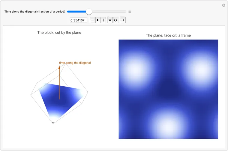
    Try it: move the slider: the plane rises through the block

    The block, cut by the plane

    The plane, face on: a frame

    The block is , on each frame.

    Mathematica
    (* The block and the plane: the cube of Cos[X]+Cos[Y]+Cos[Z] cut by the plane X+Y+Z = const, and the same cut face on, a frame of the film. On the M5: about 2 s to appear, 0.4 s per slider position. *)
    bpF[bpX_, bpY_, bpZ_] := Cos[bpX] + Cos[bpY] + Cos[bpZ];
    bpBlue[bpV_] := Blend[{RGBColor[30/255, 42/255, 130/255], RGBColor[64/255, 84/255, 206/255],
        RGBColor[150/255, 170/255, 240/255], RGBColor[245/255, 248/255, 1]}, (bpV + 3/2)/(9/2)];
    (* A point of the plane at time bpT (a fraction of a period), from its place {bpx, bpy} in the frame: three waves at 120 degrees. *)
    bpOnPlane[{bpx_, bpy_}, bpT_] := With[{bpJ = 2 bpy/Sqrt[3], bpI = bpx + bpy/Sqrt[3]},
       2 Pi ({bpI, bpJ - bpI, -bpJ} + bpT)];
    bpWaves[bpx_?NumericQ, bpy_?NumericQ, bpT_?NumericQ] := bpF @@ bpOnPlane[{bpx, bpy}, bpT];
    bpLook = Sequence[ColorFunctionScaling -> False, Mesh -> None, BoundaryStyle -> None, PlotPoints -> 60,
       PerformanceGoal -> "Quality"];
    (* The cube below the plane: its three outer faces, darker, and the cut, X+Y+Z = 6 Pi bpT. *)
    bpBlock[bpT_] := With[{bpC = 6 Pi bpT}, Show[
        ParametricPlot3D[{{2 Pi, bpU, bpV}, {bpU, 2 Pi, bpV}, {bpU, bpV, 2 Pi}}, {bpU, 0, 2 Pi}, {bpV, 0, 2 Pi},
         RegionFunction -> (#1 + #2 + #3 <= bpC &), ColorFunction -> (Darker[bpBlue[bpF[#1, #2, #3]], 0.3] &),
         Evaluate[bpLook]],
        ParametricPlot3D[{bpU, bpV, bpC - bpU - bpV}, {bpU, 0, 2 Pi}, {bpV, 0, 2 Pi},
         RegionFunction -> (0 <= #3 <= 2 Pi &), ColorFunction -> (bpBlue[bpF[#1, #2, #3]] &), Evaluate[bpLook]],
        Graphics3D[{FaceForm[], EdgeForm[GrayLevel[0.6]], Cuboid[{0, 0, 0}, {2 Pi, 2 Pi, 2 Pi}],
          RGBColor[0.75, 0.35, 0], Thickness[0.006], Arrowheads[0.04], Arrow[{{-1, -1, -1}, {8, 8, 8}}],
          Text["time along the diagonal", {8, 8, 8}, {-1, -1.5}]}],
        PlotRange -> {{-1.2, 9}, {-1.2, 9}, {-1.2, 9}}, Lighting -> {{"Ambient", White}}, Axes -> False, Boxed -> False,
        ViewPoint -> 3 {0.93, 0.33, 0.16}, ViewVertical -> {1, 1, 1}, ViewProjection -> "Orthographic",
        ImageSize -> 340, PlotLabel -> "The block, cut by the plane"]];
    bpFrame[bpT_] := DensityPlot[bpWaves[bpx, bpy, bpT], {bpx, -3/4, 3/4}, {bpy, -3/4, 3/4}, PlotRange -> All,
       ColorFunction -> bpBlue, ColorFunctionScaling -> False, PlotPoints -> 120, MaxRecursion -> 0,
       PerformanceGoal -> "Quality", Frame -> False, ImageSize -> 340, PlotLabel -> "The plane, face on: a frame"];
    Manipulate[Row[{bpBlock[bpTime], bpFrame[bpTime]}, Spacer[10]],
     {{bpTime, N[34/96], "Time along the diagonal (fraction of a period)"}, 0., 1., 1/96., Appearance -> "Open"},
     SaveDefinitions -> True]
    

    Download block-plane.wl

    The cube of cos X + cos Y + cos Z cut by a plane, beside the cut seen face on, with a time slider.
    What this draws, in Wolfram 15.0, 00:02

    Time keeps its direction, so the film's symmetry groups are the 68 . On 17 every cost is 0: a still picture's group, repeated. On the other 51, space and time .

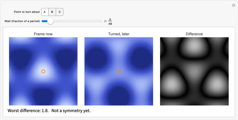
    Try it: pick a point, then wind the wait until the difference goes black

    Frame now

    Turned, later

    Difference

    Mathematica
    (* Move, then wait: the frame now, the film turned 120 degrees about a point and read after the wait, and their difference, black when the two agree. On the M5: about 1 s to appear, 0.2 s per slider position. *)
    (* The three-wave film in triangular coordinates: x = i - j/2, y = j Sqrt[3]/2, phase th = 2 Pi t/T. *)
    mwFilm[mwI_, mwJ_, mwTh_] := Cos[2 Pi mwI - mwTh] + Cos[2 Pi (mwJ - mwI) - mwTh] + Cos[-2 Pi mwJ - mwTh];
    (* The turn about {ci, cj}, clockwise. *)
    mwTurn[{mwCi_, mwCj_}, mwI_, mwJ_] := {-(mwI - mwCi) + (mwJ - mwCj) + mwCi, -(mwI - mwCi) + mwCj};
    mwPoints = <|"A" -> {0, 0}, "B" -> {2/3, 0}, "C" -> {1/3, 0}|>;
    mwBlue[mwV_] := Blend[{RGBColor[30/255, 42/255, 130/255], RGBColor[64/255, 84/255, 206/255],
        RGBColor[150/255, 170/255, 240/255], RGBColor[245/255, 248/255, 1]}, (mwV + 3/2)/(9/2)];
    (* The window of the plane around the point, 1.5 across and 150 by 150, as arrays of i and j. *)
    mwWindow[{mwCi_, mwCj_}] := With[{mwXs = (mwCi - mwCj/2) + Subdivide[-0.75, 0.75, 149],
        mwYs = Sqrt[3.]/2 mwCj + Subdivide[0.75, -0.75, 149]},
       With[{mwJs = Transpose[ConstantArray[mwYs/(Sqrt[3.]/2), 150]]}, {ConstantArray[mwXs, 150] + mwJs/2, mwJs}]];
    (* Now, turned and later, and their absolute difference: q(g x, t + wait T) = q(x, t) when the wait is the move's cost. *)
    mwArrays[mwP_, mwWait_] := With[{mwC = mwPoints[mwP], mwTh = 0.5}, With[{mwW = mwWindow[mwC]},
        With[{mwA = mwFilm[mwW[[1]], mwW[[2]], mwTh],
          mwB = mwFilm[Sequence @@ mwTurn[mwC, mwW[[1]], mwW[[2]]], mwTh + 2. Pi mwWait]}, {mwA, mwB, Abs[mwA - mwB]}]]];
    mwPanel[mwTitle_, mwData_, mwColor_, mwRing_] := ArrayPlot[mwData, ColorFunction -> mwColor,
       ColorFunctionScaling -> False, DataRange -> {{-0.75, 0.75}, {-0.75, 0.75}}, Frame -> False, ImageSize -> 230,
       PlotLabel -> mwTitle, Epilog -> If[mwRing, {Orange, Thick, Circle[{0, 0}, 0.035]}, {}]];
    mwShow[mwP_, mwWait_] := With[{mwAll = mwArrays[mwP, mwWait]}, Column[{
        Row[{mwPanel["Frame now", mwAll[[1]], mwBlue, True], mwPanel["Turned, later", mwAll[[2]], mwBlue, True],
          mwPanel["Difference", mwAll[[3]], GrayLevel[#/2.5] &, False]}, Spacer[6]],
        Style[Row[{"Worst difference: ", NumberForm[Max[mwAll[[3]]], 2], If[Max[mwAll[[3]]] < 10^-9,
            Row[{".   Black: the turn about ", mwP, " costs ", mwWait, " of a period."}], ".   Not a symmetry yet."]}], "Text"]}]];
    Manipulate[mwShow[mwPoint, mwWait],
     {{mwPoint, "A", "Point to turn about"}, Keys[mwPoints], SetterBar},
     {{mwWait, 5/48, "Wait (fraction of a period)"}, 0, 1, 1/48, Appearance -> "Labeled"},
     SaveDefinitions -> True]
    

    Download move-wait.wl

    Point chips and a wait slider over three panels: the frame now, the frame turned and later, and their difference.
    What this draws, in Wolfram 15.0, 00:01

    So each move has its own cost: the turn about A is free, about B a third of a period, about C two thirds. Those three turns make the plane group 333 into the crystal r33₁3₂: writes the costs as subscripts.

    68 crystal types, 71 labellings

    Independently classified as a plane group plus a cost on each of its moves: 68 crystal types by point group (rotations and mirrors alone), 1: 1; 2: 3; m: 4; mm2: 22; 4: 6; 4mm: 12; 3: 4; 3m: 6; 6: 6; 6mm: 4. Four mirror-image pairs are counted apart. Counted as labellings it is 71. The three extras, all in point group m, are real films on a crystal that one of the 68 already names, with time along another axis of that crystal:

    • On , both mirror families cost . Each mirror becomes a glide along time: crystal Pc, named by ××.
    • On , one mirror family is free and the other costs ; put another way, a translation across the mirrors costs : crystal Cm, named by *×.
    • On , a translation across the glides costs : crystal Cc, named by ~*×½.

    As films each differs from the one named; as crystals they are the same. The site's section Relabelling explains this on the first of them, and why it counts them as one: it allows any re-basing of the lattice, and that is where its count of 275 and the stricter 283 part. Conway and coauthors (table 2b) list each pair as two names for one crystal: and for Pc, and for Cm, and for Cc. Source: an independent check of the geometry, in part2-numbers.json.

    A cost on a translation alone is only a drift

    "Do not decompose" in full: no frames , with left alone by every rotation and mirror, put all the spatial moves inside one frame. A translation that costs time alone is only a drift: tilting the frames removes the cost. It becomes a real cost when a rotation or mirror forbids the tilt. In r33₁3₂ the turns about the pure axes cost nothing, and the cost sits on the translations. Source: an independent check of the geometry, in part2-numbers.json.

    10. The one change to SymSim

    His of section 5 reads now. Section 9's relation says when to read it for a film: if the move carries out to , the value at now is the value at , ago. With :

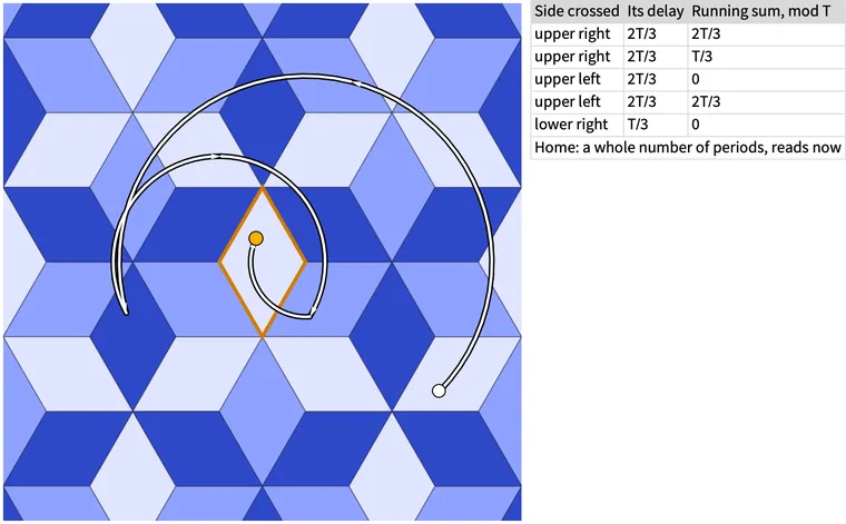
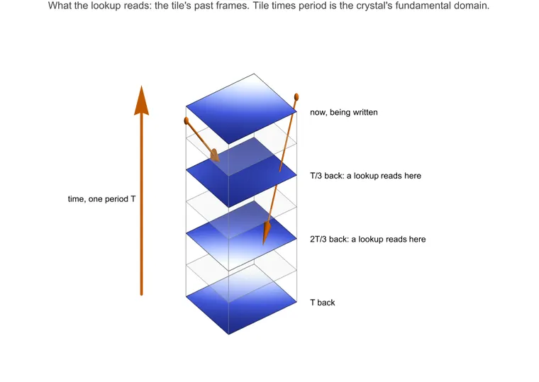
    It takes one new number per side of the tile, its delay: the cost of the move that carries the tile out across that side. On the way home the delays add along the , modulo a whole period, and the sum is , which depends on the pixel. The equation and the grid stay. Two things come with it: a stack of past frames to read, and itself (section 13).

    Try it: tap a point and add up its delays

    reads now ago ago

      The white path is the word of moves, as in section 2. Each row: a side crossed, its delay, the running sum. The last row is what the pixel reads.

      Mathematica
      (* The word and its delays: the plane tiled by the 333 rhombus, each copy tinted by how long ago it reads. Drag the point: the white path of moves folds it home, and the table adds up their delays. On the M5: under a second to appear, 0.1 s per position of the point. *)
      (* The rhombus and its four sides, in his order: a point is outside a side when normal . point > Sqrt[3]/4. *)
      wdSides = N[{{Sqrt[3], 1}, {-Sqrt[3], 1}, {Sqrt[3], -1}, {-Sqrt[3], -1}}/2];
      wdNames = {"upper right", "upper left", "lower right", "lower left"};
      wdPivots = {{1/2, 0}, {-1/2, 0}, {1/2, 0}, {-1/2, 0}};
      wdAngles = {1, -1, -1, 1} 2 Pi/3;
      wdDelays = {2/3, 2/3, 1/3, 1/3};
      wdMoves = N[MapThread[RotationTransform, {wdAngles, wdPivots}]];
      wdRhombus = N[{{0, -Sqrt[3]/2}, {1/2, 0}, {0, Sqrt[3]/2}, {-1/2, 0}}];
      (* His fold: the first side the point is outside moves it; start the sides over. 0 means home. *)
      wdSide[wdP_] := First[FirstPosition[wdSides . wdP, _?(# > Sqrt[3.]/4 + 10^-7 &), {0}, {1}]];
      wdStops[wdP_] := NestWhileList[wdMoves[[wdSide[#]]][#] &, N[wdP], wdSide[#] > 0 &];
      wdWord[wdP_] := wdSide /@ Most[wdStops[wdP]];
      wdDelay[wdP_] := Mod[Total[wdDelays[[wdWord[wdP]]]], 1];
      (* Every copy of the tile in view: its three turns about {1/2, 0}, slid along the group's two translations. *)
      wdCopies = N[Flatten[Table[(# + wdN {3/2, Sqrt[3]/2} + wdM {0, Sqrt[3]}) & /@
            (RotationTransform[wdK 2 Pi/3, {1/2, 0}] /@ wdRhombus), {wdK, 0, 2}, {wdN, -3, 3}, {wdM, -4, 4}], 2]];
      wdTint = <|0 -> RGBColor[223/255, 229/255, 1], 1/3 -> RGBColor[143/255, 162/255, 1], 2/3 -> RGBColor[47/255, 73/255, 200/255]|>;
      wdPlane = {EdgeForm[RGBColor[0.08, 0.09, 0.24, 0.45]], {wdTint[wdDelay[Mean[#]]], Polygon[#]} & /@ wdCopies,
         {EdgeForm[{Opacity[1], RGBColor[0.82, 0.48, 0], Thickness[0.007]}], FaceForm[], Polygon[wdRhombus]}};
      wdArc[wdS_, wdP_] := Table[RotationTransform[wdAngles[[wdS]] wdU, wdPivots[[wdS]]][wdP], {wdU, 0, 1, 1/24}];
      wdPicture[wdP_] := With[{wdPath = wdStops[wdP], wdArcs = MapThread[wdArc, {wdWord[wdP], Most[wdStops[wdP]]}]},
         Graphics[{wdPlane, Arrowheads[0.02], CapForm["Round"], {Black, Thickness[0.011], Line[wdArcs]},
           {White, Thickness[0.005], Arrow /@ wdArcs}, {EdgeForm[Black], RGBColor[1, 0.69, 0], Disk[Last[wdPath], 0.08]}},
          PlotRange -> {{-3, 3}, {-3, 3}}, ImageSize -> 480]];
      wdFrac[wdQ_] := Which[wdQ == 0, 0, wdQ == 1/3, "T/3", wdQ == 2/3, "2T/3"];
      wdTable[wdP_] := With[{wdW = wdWord[wdP]}, Style[Grid[Join[{{"Side crossed", "Its delay", "Running sum, mod T"}},
            MapThread[{#1, wdFrac[#2], wdFrac[Mod[#3, 1]]} &, {wdNames[[wdW]], wdDelays[[wdW]], Accumulate[wdDelays[[wdW]]]}],
            {{Which[wdW === {}, "Inside the tile: it reads itself, now", wdDelay[wdP] == 0, "Home: a whole number of periods, reads now",
               True, Row[{"Home: reads the tile ", wdFrac[wdDelay[wdP]], " ago"}]], SpanFromLeft, SpanFromLeft}}],
           Alignment -> Left, Frame -> All, FrameStyle -> LightGray, Background -> {None, {LightGray}}], "Text"]];
      DynamicModule[{wdPoint = {2.05, -1.5}}, Grid[{{
          LocatorPane[Dynamic[wdPoint], Dynamic[wdPicture[wdPoint]], Appearance -> Graphics[{EdgeForm[Black], White, Disk[]}, ImageSize -> 14]],
          Dynamic[wdTable[wdPoint]]}}, Alignment -> Top], SaveDefinitions -> True]
      

      Download word-delays.wl

      The plane tiled by the rhombus, each copy tinted by its delay, beside a table of sides, delays and the running sum.
      What this draws, in Wolfram 15.0, 00:01
      timenow⅓ period ago⅔ period ago1 period ago
      What reads: the tile's past frames, deep here. Tile times period is the crystal's fundamental domain.
      Mathematica
      (* The prism: the tile times the period. The rhombus at the bottom, past frames stacked to height T, the frame being written on top, the slices a lookup reads marked T/3 and 2T/3 back. On the M5: about a second. *)
      (* The film on this rhombus: section 9's three waves turned 60 degrees, its free axis on the top corner; prT is time in periods. *)
      prFilm[prX_, prY_, prT_] := With[{prV = {prX, prY - Sqrt[3]/2}},
         Total[Cos[(4 Pi/(3 Sqrt[3])) {Cos[#], Sin[#]} . prV - 2 Pi prT] & /@ ({90, 210, 330} Degree)]];
      prBlue[prV_] := Blend[{RGBColor[30/255, 42/255, 130/255], RGBColor[64/255, 84/255, 206/255],
          RGBColor[150/255, 170/255, 240/255], RGBColor[245/255, 248/255, 1]}, (prV + 3/2)/(9/2)];
      prInside[prX_, prY_] := Sqrt[3] Abs[prX] + Abs[prY] <= Sqrt[3]/2;
      prCorners = {{0, -Sqrt[3]/2}, {1/2, 0}, {0, Sqrt[3]/2}, {-1/2, 0}};
      prLift[prPoly_, prZ_] := Append[#, prZ] & /@ prPoly;
      prSlice[prZ_] := ParametricPlot3D[{prX, prY, prZ}, {prX, -1/2, 1/2}, {prY, -Sqrt[3]/2, Sqrt[3]/2},
         RegionFunction -> (prInside[#1, #2] &), ColorFunction -> (prBlue[prFilm[#1, #2, prZ]] &), ColorFunctionScaling -> False,
         Mesh -> None, BoundaryStyle -> Black, PlotPoints -> 50, Lighting -> "Neutral"];
      (* Two pixels just outside the tile, on the frame being written, and where each reads: its one move and that side's delay. *)
      prLookups = {{{-0.45, -0.35}, 2 Pi/3, {-1/2, 0}, 1/3}, {{0.45, 0.35}, 2 Pi/3, {1/2, 0}, 2/3}};
      prArrow[{prP_, prAngle_, prPivot_, prTau_}] := {Arrowheads[0.025],
         Arrow[Tube[{Append[prP, 1], Append[RotationTransform[prAngle, prPivot][prP], 1 - prTau]}, 0.007]],
         Sphere[Append[prP, 1], 0.02]};
      Show[prSlice /@ {0, 1/3, 2/3, 1}, Graphics3D[{
          {Opacity[0.25], LightGray, EdgeForm[Gray], Polygon[prLift[prCorners, #]] & /@ {1/6, 1/2, 5/6}},
          {Gray, Line[{Append[#, 0], Append[#, 1]}] & /@ prCorners},
          {RGBColor[0.75, 0.35, 0], prArrow /@ prLookups},
          {RGBColor[0.75, 0.35, 0], Thickness[0.005], Arrowheads[0.03], Arrow[{{-0.9, 0, 0}, {-0.9, 0, 1.1}}],
           Black, Text["time, one period T", {-0.95, 0, 1/2}, {1, 0}]},
          MapThread[Text[#1, {0.62, 0, #2}, {-1, 0}] &, {{"now, being written", "T/3 back: a lookup reads here",
             "2T/3 back: a lookup reads here", "T back"}, {1, 2/3, 1/3, 0}}]}],
       PlotRange -> {{-1.8, 2.3}, {-1, 1}, {-0.05, 1.15}}, BoxRatios -> {2.05, 1, 1.1}, Boxed -> False, Axes -> False,
       ViewPoint -> {0.4, -3, 1.2}, ViewProjection -> "Orthographic", ImageSize -> 640,
       PlotLabel -> "What the lookup reads: the tile's past frames. Tile times period is the crystal's fundamental domain."]
      

      Download prism.wl

      The rhombus at the bottom of a prism of past frames, with two lookup arrows reading T/3 and 2T/3 back.
      What this draws, in Wolfram 15.0, 00:01
      His fold needs no new code: two z-planes per side

      His fold works on 3D points. Add two horizontal planes to a side's word and each pass through that side moves pnt.z by minus that side's delay:

      words.map((w, i) => [...w, iPlane([0,0,1,0]), iPlane([0,0,1,-taus[i]/2])])

      Run through his unedited shader in headless Chrome, 16,384 points: exactly as the plain group (worst difference 0.0), equal, modulo 1, to the group's cost over all 83 fold words. On the published film, every node from the rhombus's own past: residual 0.0; ignoring , 1.846. Source: an independent check of the geometry, in part2-numbers.json. The diff: patch-a-phase-twist.diff.

      Side delays. On his side order, , with section 9's film turned onto this rhombus and its free axis on a corner (worst , 5,000 points). Left unturned, the same film needs . A pair's delays add to exactly one period, not zero, and that period is what keeps both sides in the past. Delays needed reach , not .

      A trap. The fold leaves in the closed interval from to 0, and in float32 912 of 5,384 whole-period grid points read just under a whole number, so fract(-z) reads a period ago. On a settled film that is the same frame; during a transient it is not. Round to the group's denominator.

      The prism, exactly

      The stack of past frames is the crystal being written. Neighbouring prisms are staggered like bricks by , so whole walls pair only once cut at thirds of . At the pure corners (A's kind, where the turn is free) two edges glue to one circle of cone angle , one period long; at the other two corners one edge is cut into three pieces totalling , an ordinary line. The history is this prism only once the film has settled, and only its tile part. Source: an independent check of the geometry, in part2-numbers.json.

      11. Check on the Brusselator

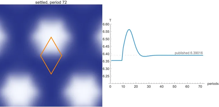
      The test is the film of the clockwork orbits tutorial, from the Brusselator, a different pair of chemicals:

      with . Only the group goes in: white noise on the tile, a guess for .

      Try it: press Play and watch the film form; the switch changes what the reads

      period 0 -

      The plane, tile outlined. Until it settles, copies darken with age

      against periods

      This runs on the published film's triangular mesh, one lookup a step. Section 14 runs his pixels.

      Mathematica
      (* The delayed lookup from white noise: the film forms on the plane, tile outlined, beside T against periods with the published 6.39016 dashed. Set glueLookupReadsPast = False and the copies read now, so the plane collapses to one tick, T = 6.4276. 45 s on the M5. *)
      glueLookupReadsPast = True;
      SeedRandom[1];
      {glueN, glueL, glueA, glueB, gluePer} = {36, 40., 1., 2.3, 336};
      glueLap[f_] := 2/(3 (glueL/glueN)^2) ListCorrelate[{{1, 1, 0}, {1, -6, 1}, {0, 1, 1}}, f, {2, 2}];
      glueF[q_] := With[{u = q[[1]], v = q[[2]], r = q[[1]]^2 q[[2]]},
         {glueLap[u] + glueA - (glueB + 1) u + r, glueLap[v] + glueB u - r}];
      glueRK4[q_, h_] := Module[{k1 = glueF[q], k2, k3},
         k2 = glueF[q + h/2 k1];
         k3 = glueF[q + h/2 k2];
         q + h/6 (k1 + 2 k2 + 2 k3 + glueF[q + h k3])];
      glueOps = Flatten[Table[{Inverse[m], s[[1]], s[[2]]},
          {m, {{{1, 0}, {0, 1}}, {{-1, 1}, {-1, 0}}, {{0, -1}, {1, -1}}}},
          {s, {{{0, 0}, 0}, {{12, 24}, 2}, {{24, 12}, 1}}}], 1];
      glueOutside[{x_, y_}] := Min@Table[Max[Abs[3 (x/glueN + i) - 1/2], Abs[3 ((y - x)/glueN + j) - 1/2]], {i, -1, 1}, {j, -1, 1}];
      glueSource[p_] := First@Sort@Table[With[{r = Mod[g[[1]].(p - g[[2]]), glueN]},
           {glueOutside[r], r[[2]] glueN + r[[1]] + 1, g[[3]]}], {g, glueOps}];
      glueLookup = Flatten@Table[With[{s = glueSource[{x, y}]}, s[[2]] + If[glueLookupReadsPast, s[[3]] glueN^2, 0]],
          {y, 0, glueN - 1}, {x, 0, glueN - 1}];
      glueHopf = 2 Pi/Sqrt[glueA^2 - ((glueB - 1 - glueA^2)/2)^2];
      glueQ = {ConstantArray[glueA, {glueN, glueN}], ConstantArray[glueB/glueA, {glueN, glueN}]} + RandomVariate[NormalDistribution[0, 0.1], {2, glueN, glueN}];
      glueHist = ConstantArray[Flatten[glueQ, {{1}, {2, 3}}], gluePer];
      {glueT, glueI, glueTime, glueLast, glueLevel, glueDrift, glueTs, glueFields} = {glueHopf, 0, 0., None, None, 1., {}, {}};
      glueStep[] := Module[{old = glueQ[[1, 1, 1]], new, f, dt = glueT/gluePer},
         f = Flatten[glueRK4[glueQ, dt], {{1}, {2, 3}}];
         f = Join[f, glueHist[[Mod[glueI + 1 - gluePer/3, gluePer, 1]]], glueHist[[Mod[glueI + 1 - 2 gluePer/3, gluePer, 1]]], 2][[All, glueLookup]];
         glueI++; glueTime += dt;
         glueDrift = Sqrt[Mean[Flatten[(f - glueHist[[Mod[glueI, gluePer, 1]]])^2]]];
         glueHist[[Mod[glueI, gluePer, 1]]] = f;
         glueQ = ArrayReshape[f, {2, glueN, glueN}];
         new = f[[1, 1]];
         If[NumberQ[glueLevel] && old < glueLevel <= new,
          With[{cross = glueTime - dt (new - glueLevel)/(new - old)},
           If[NumberQ[glueLast] && 0.7 glueHopf < cross - glueLast < 1.4 glueHopf, glueT = cross - glueLast];
           glueLast = cross]];
         If[Mod[glueI, gluePer] == 0,
          With[{r = MinMax[glueHist[[All, 1, 1]]]}, glueLevel = If[r[[2]] - r[[1]] > 0.1, Mean[r], None]];
          AppendTo[glueTs, glueT]];];
      glueSave[label_] := AppendTo[glueFields, {label, ArrayReshape[glueHist[[Mod[glueI, gluePer, 1], 1]], {glueN, glueN}]}];
      Monitor[
        glueSave["period 0"];
        While[Length[glueTs] < 300 && (Length[glueTs] < 20 || glueDrift > 1*^-8),
         glueStep[];
         If[Length[glueTs] < 24 && Mod[glueI, gluePer/8] == 0, glueSave["period " <> ToString[NumberForm[N[glueI/gluePer], {3, 1}]]]]];
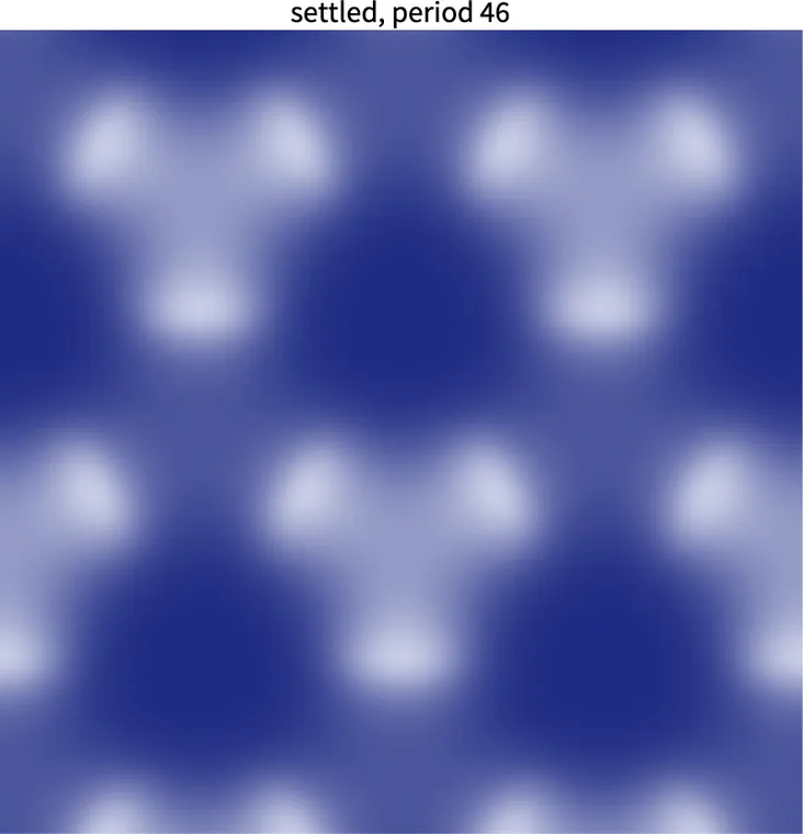
        Do[glueStep[]; If[Mod[s, gluePer/48] == 0, glueSave["settled, period " <> ToString[Length[glueTs]]]], {s, gluePer}],
        Row[{"period ", Length[glueTs], "   T = ", glueT, "   drift ", glueDrift}]];
      glueRange = MinMax[Last /@ Take[glueFields, -48]];
      glueRange = If[Subtract @@ Reverse[glueRange] < 0.4, Mean[glueRange] + {-0.2, 0.2}, glueRange];
      {glueGridI, glueGridJ} = Transpose[Table[With[{x = 32 ((c - 1/2)/120 - 1), y = 11.55 + 32 (1 - (r - 1/2)/120)}, {x/glueL + y/(Sqrt[3.] glueL), 2 y/(Sqrt[3.] glueL)}], {r, 240}, {c, 240}], {2, 3, 1}];
      glueImage[u_] := Image[Image[Threaded[{30, 42, 130}/255.] + TensorProduct[Clip[ListInterpolation[ArrayPad[Rescale[u, glueRange], {{0, 1}, {0, 1}}, "Periodic"], {{0., 1.}, {0., 1.}},
              PeriodicInterpolation -> True, InterpolationOrder -> 3][glueGridJ, glueGridI], {0., 1.}], {215, 206, 125}/255.]], "Byte"];
      gluePicture[{label_, u_}] := Graphics[{
          Inset[glueImage[u],
           {-32., -20.45}, {Left, Bottom}, {64., 64.}],
          Orange, Thick, Line[glueL {{0, 0}, {1/6, Sqrt[3.]/6}, {0, Sqrt[3.]/3}, {-1/6, Sqrt[3.]/6}, {0, 0}}]},
         PlotLabel -> label, ImageSize -> 300, PlotRange -> {{-32., 32.}, {-20.45, 43.55}}, PlotRangePadding -> 0];
      glueFrames = gluePicture /@ glueFields;
      Print["T = ", glueT, " after ", Length[glueTs], " periods; spread of u across the plane ", StandardDeviation[Flatten[glueFields[[-1, 2]]]]];
      Row[{ListAnimate[glueFrames, 12],
        ListLinePlot[glueTs, PlotRange -> {6.2, 6.6}, AxesLabel -> {"periods", "T"}, ImageSize -> 340,
         GridLines -> {None, {{6.39016, Directive[Dashed, Gray]}}},
         Epilog -> Text[Style["published 6.39016", Gray], {Length[glueTs], 6.39016}, {1, -1.3}]]}]
      

      Download glue-film.wl

      The settled film on the plane, tile outlined, beside T against periods, closing on the dashed published value.
      What this draws, in Wolfram 15.0, 00:47
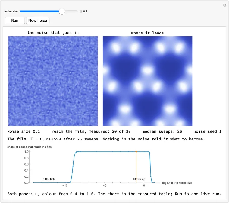
      The numbers: 12 of 12 seeds land on the published film

      An independent simulator, written from the mathematics: 12 of 12 seeds from noise, within of the published , distance at most, the rounding of the stored film. Noise 1.0, noise in the history too, a random tile: 3 of 3, 3 of 3, 3 of 3. 50 to 59 periods. Source: an independent check of the dynamics, in part2-numbers.json.

      This demo, the page's JavaScript timing one pixel, as in section 13: 12 of 12 seeds, 67 to 72 periods until 's drift is under , within , distance to , limited by the 48 stored frames' interpolation. The live readout compares only, and this demo's tile is his rhombus, not that simulator's cut. Code: glue-film.mjs; source: part2-measure.json.

      The switch. Reading now instead of the past, same noise: the spread of , its standard deviation across the plane, is under by period 20, 6 of 6 seeds, every cell ticking together with period .

      A slow phone. If a step takes too long, Restart uses or in place of , and the readout says which. lands on that mesh's own value, and , with no distance to read. It takes about 0.05 ms a step here on a laptop. No real phone was timed.

      How often must the lookup run?

      Rarely, as his slide says: "once per 1000 simulation steps" (JMM 2024, slide 121). With all cells evolving and the copies overwritten every steps: 2 of 2 land at (3 periods apart), 0 of 2 at . The plain mesh regrows the unison mode a period and one overwrite keeps about 3 to 4% of it, which crosses at , 22 periods. Source: an independent check of the dynamics, in part2-numbers.json.

      12. Why it now works

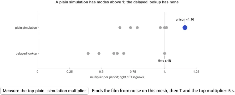
      Left alone, the film is unstable: all cells drift into ticking together, the unison mode, which grows a period, its . His symmetrization cannot stop it, since a field ticking in unison obeys every same-moment symmetry. The delayed lookup removes it: a mode that grows cannot equal its own past.

      A plain simulation has modes above 1; the delayed lookup has none

      00.250.50.7511.25multiplier per period; right of 1 it growsplain simulationdelayed lookupunison ×1.16time shift

      One cut of the tile (where its sides are drawn), frozen. Time shift: the film's clock can start at any moment, so a multiplier of 1 is always there.

      Mathematica
      (* Multipliers per period, plain simulation against the delayed lookup, with the line at 1. On the M5: the chart in 2 s; its button measures the top plain-simulation multiplier here, from noise, in 5 s. *)
      (* Typed in: the largest multipliers per period of the published 333 Brusselator film on the triangular mesh N = 36, box 40, T frozen. Plain simulation: the map over one period. Delayed lookup: the same film under the lookup, on one cut of the tile. *)
      mlPlain = {1.1608, 1.1608, 1.0153, 1.0153, 1.0153, 1.0153, 1.0000, 1.0000, 1.0000, 0.9666, 0.9666, 0.7847, 0.7847, 0.7311, 0.7311, 0.6470};
      mlLookup = {1.0000, 0.6769, 0.6267, 0.5988, 0.4817, 0.3965, 0.3965, 0.3961};
      mlChart = ListPlot[{Thread[{mlPlain, 2}], Thread[{mlLookup, 1}], {Callout[{First[mlPlain], 2}, "unison \[Times]1.16", Above]}, {Callout[{1, 1}, "time shift", Below]}},
         PlotStyle -> {{PointSize[0.018], GrayLevel[0.65]}, {PointSize[0.018], GrayLevel[0.65]}, {PointSize[0.03], RGBColor[0.19, 0.29, 0.78]}, {PointSize[0.018], GrayLevel[0.65]}},
         GridLines -> {{{1, Directive[Gray]}}, None}, PlotRange -> {{0, 1.25}, {0.4, 2.6}}, Frame -> {True, True, False, False},
         FrameTicks -> {{{{1, "delayed lookup"}, {2, "plain simulation"}}, None}, {Range[0, 1.25, 0.25], None}},
         FrameLabel -> {"multiplier per period; right of 1 it grows", None},
         PlotLabel -> Style["A plain simulation has modes above 1; the delayed lookup has none", Bold],
         AspectRatio -> 0.36, ImageSize -> 640, ImagePadding -> {{120, 20}, {50, 25}}];
      (* The Brusselator on the mesh, RK4, the slide that costs T/3, and one sweep: a free period, three frames, slide back, average, correct T. *)
      mlLap[mlQ_] := (2/3) (36/40.)^2 (RotateLeft[mlQ, {0, 0, 1}] + RotateLeft[mlQ, {0, 0, -1}] + RotateLeft[mlQ, {0, 1, 0}] +
           RotateLeft[mlQ, {0, -1, 0}] + RotateLeft[mlQ, {0, 1, 1}] + RotateLeft[mlQ, {0, -1, -1}] - 6 mlQ);
      mlF[mlQ_] := mlLap[mlQ] + {1 - 3.3 mlQ[[1]] + mlQ[[1]]^2 mlQ[[2]], 2.3 mlQ[[1]] - mlQ[[1]]^2 mlQ[[2]]};
      mlFlow[mlQ_, mlT_] := With[{mlH = mlT/Ceiling[mlT/0.02]}, Nest[Function[mlS, Module[{mlA = mlF[mlS], mlB, mlC},
            mlB = mlF[mlS + mlH/2 mlA]; mlC = mlF[mlS + mlH/2 mlB];
            mlS + mlH/6 (mlA + 2 mlB + 2 mlC + mlF[mlS + mlH mlC])]], mlQ, Ceiling[mlT/0.02]]];
      mlSlide[mlQ_] := RotateLeft[mlQ, {0, 12, 24}];
      mlTurn[mlQ_] := Table[mlQ[[mlC, Mod[mlX - mlY, 36] + 1, Mod[-mlY, 36] + 1]], {mlC, 2}, {mlY, 0, 35}, {mlX, 0, 35}];
      mlSweep[{mlQ_, mlT_}] := Module[{mlA = mlFlow[mlQ, mlT], mlB, mlC, mlR, mlV},
         mlB = mlFlow[mlA, mlT/3]; mlC = mlFlow[mlB, mlT/3]; mlR = mlSlide[mlB] - mlA; mlV = mlF[mlA];
         {(mlA + mlSlide[mlB] + mlSlide[mlSlide[mlC]])/3, mlT - Clip[3 Total[mlR mlV, 3]/Total[mlV mlV, 3], {-0.1, 0.1}]}];
      (* The film from noise, then a uniform kick pushed through the linearized period map. The top mode is a slowly turning pair, so its size comes from three successive kicks: v2 = a v1 + b v0, |mu|^2 = -b. *)
      mlMeasure[] := Module[{mlFilm, mlT, mlNext, mlMap, mlKick, mlAfter, mlFit},
         SeedRandom[1];
         {mlFilm, mlT} = Nest[mlSweep, {With[{mlN = {1., 2.3} + 0.1 RandomVariate[NormalDistribution[], {2, 36, 36}]},
             (mlN + mlTurn[mlN] + mlTurn[mlTurn[mlN]])/3], 6.355}, 30];
         mlNext = mlFlow[mlFilm, mlT];
         mlMap[mlV_] := (mlFlow[mlFilm + 10.^-5 mlV, mlT] - mlNext)/10.^-5;
         mlKick = Nest[With[{mlW = mlMap[#]}, mlW/Norm[Flatten[mlW]]] &, ConstantArray[1./Sqrt[2592.], {2, 36, 36}], 60];
         mlAfter = mlMap[mlKick];
         mlFit = LeastSquares[Transpose[{Flatten[mlAfter], Flatten[mlKick]}], Flatten[mlMap[mlAfter]]];
         <|"T" -> mlT, "top multiplier" -> Sqrt[-mlFit[[2]]], "its turn per period, degrees" -> ArcCos[mlFit[[1]]/(2 Sqrt[-mlFit[[2]]])]/Degree|>];
      DynamicModule[{mlReadout = "Finds the film from noise on this mesh, then T and the top multiplier: 5 s."}, Column[{mlChart, Row[{
           Button["Measure the top plain-simulation multiplier", mlReadout = "Running ...";
            mlReadout = Row[{"T = ", NumberForm[#T, 8], "   top multiplier = ", NumberForm[#["top multiplier"], 5]}] &[mlMeasure[]], Method -> "Queued"],
           Spacer[10], Style[Dynamic[mlReadout], "Text"]}]}], SaveDefinitions -> True]
      

      Download multipliers.wl

      Multipliers per period, the plain simulation against the delayed lookup, with the line at 1.
      What this draws, in Wolfram 15.0, 00:02
      What is proved here, and what is only measured

      The plain mesh. A mode has , with the move and the multiplier of a third of a period. The copy rule says the value across a side is the one from ago, while the mode has grown by since. So it can hold only for . Seeded under the delayed lookup, the unison mode dies 0.63 to 0.66 a period; on the plain mesh it grows 1.15 to 1.17. Source: an independent check of the dynamics, in part2-numbers.json.

      The rest is a measurement. This says why the unison mode cannot carry over, not that the lookup is stable. The system with the lookup is a delay equation, whose state is the tile plus its recent past, and it has its own modes: on the cut in the picture , , , . The plain simulation's other four multipliers above 1, all 1.0153, break the 3-fold, which any symmetrization imposes. The next mode depends on where the tile is cut, 0.667 to 0.919 over 7 cuts, stable on every one tried. With in the loop the rate is 0.62 to 0.76, depending on where in the period is read.

      13. The new knob:

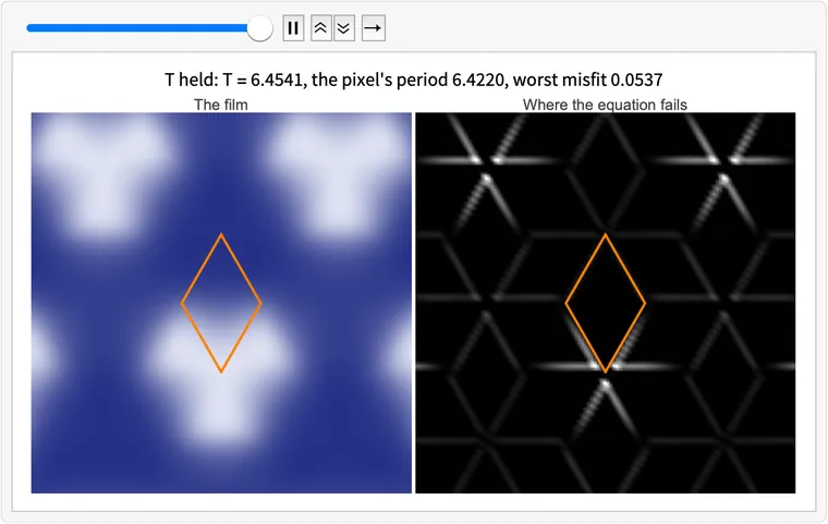
      The tile's size is yours to pick. The crystal's height is not: the symmetry leaves free, the equation fixes it. Set it wrong and the film stays periodic, with a , and its own period falls between your and the true one.

      Try it: move off, then let the film set it

      - -

      The film

      Where the equation fails

      Mathematica
      (* T held off by a fraction: the film beside the map of where the equation fails, |du/dt - right-hand side|, black where it holds. A line prints the T set, the film's own period and the worst misfit; then T is read from the film and the misfit falls to the level of the finite differences. 1 min on the M5. *)
      wtOff = 0.01;
      SeedRandom[1];
      {wtN, wtL, wtA, wtB, wtPer} = {36, 40., 1., 2.3, 336};
      wtLap[f_] := 2/(3 (wtL/wtN)^2) ListCorrelate[{{1, 1, 0}, {1, -6, 1}, {0, 1, 1}}, f, {2, 2}];
      wtF[q_] := With[{u = q[[1]], v = q[[2]], r = q[[1]]^2 q[[2]]},
         {wtLap[u] + wtA - (wtB + 1) u + r, wtLap[v] + wtB u - r}];
      wtRK4[q_, h_] := Module[{k1 = wtF[q], k2, k3},
         k2 = wtF[q + h/2 k1];
         k3 = wtF[q + h/2 k2];
         q + h/6 (k1 + 2 k2 + 2 k3 + wtF[q + h k3])];
      wtOps = Flatten[Table[{Inverse[m], s[[1]], s[[2]]},
          {m, {{{1, 0}, {0, 1}}, {{-1, 1}, {-1, 0}}, {{0, -1}, {1, -1}}}},
          {s, {{{0, 0}, 0}, {{12, 24}, 2}, {{24, 12}, 1}}}], 1];
      wtOutside[{x_, y_}] := Min@Table[Max[Abs[3 (x/wtN + i) - 1/2], Abs[3 ((y - x)/wtN + j) - 1/2]], {i, -1, 1}, {j, -1, 1}];
      wtSource[p_] := First@Sort@Table[With[{r = Mod[g[[1]].(p - g[[2]]), wtN]},
           {wtOutside[r], r[[2]] wtN + r[[1]] + 1, g[[3]]}], {g, wtOps}];
      wtLookup = Flatten@Table[With[{s = wtSource[{x, y}]}, s[[2]] + s[[3]] wtN^2], {y, 0, wtN - 1}, {x, 0, wtN - 1}];
      wtHopf = 2 Pi/Sqrt[wtA^2 - ((wtB - 1 - wtA^2)/2)^2];
      wtQ = {ConstantArray[wtA, {wtN, wtN}], ConstantArray[wtB/wtA, {wtN, wtN}]} + RandomVariate[NormalDistribution[0, 0.1], {2, wtN, wtN}];
      wtHist = ConstantArray[Flatten[wtQ, {{1}, {2, 3}}], wtPer];
      {wtT, wtI, wtTime, wtLast, wtLevel, wtDrift, wtP, wtFree} = {wtHopf, 0, 0., None, None, 1., None, True};
      wtFrame[back_] := wtHist[[Mod[wtI - back, wtPer, 1]]];
      wtStep[] := Module[{old = wtQ[[1, 1, 1]], new, f, dt = wtT/wtPer},
         f = Flatten[wtRK4[wtQ, dt], {{1}, {2, 3}}];
         f = Join[f, wtFrame[wtPer/3 - 1], wtFrame[2 wtPer/3 - 1], 2][[All, wtLookup]];
         wtI++; wtTime += dt;
         wtDrift = Sqrt[Mean[Flatten[(f - wtHist[[Mod[wtI, wtPer, 1]]])^2]]];
         wtHist[[Mod[wtI, wtPer, 1]]] = f;
         wtQ = ArrayReshape[f, {2, wtN, wtN}];
         new = f[[1, 1]];
         If[NumberQ[wtLevel] && old < wtLevel <= new,
          With[{cross = wtTime - dt (new - wtLevel)/(new - old)},
           If[NumberQ[wtLast] && 0.7 wtHopf < cross - wtLast < 1.4 wtHopf,
            wtP = cross - wtLast;
            If[wtFree, wtT = wtP]];
           wtLast = cross]];
         If[Mod[wtI, wtPer] == 0,
          With[{r = MinMax[wtHist[[All, 1, 1]]]}, wtLevel = If[r[[2]] - r[[1]] > 0.1, Mean[r], None]]];];
      wtMisfit[] := ArrayReshape[Abs[(wtFrame[0][[1]] - wtFrame[2][[1]]) wtPer/(2 wtT) - Flatten[wtF[ArrayReshape[wtFrame[1], {2, wtN, wtN}]][[1]]]], {wtN, wtN}];
      wtKeep[label_] := With[{m = wtMisfit[]},
         AppendTo[wtSaved, {label <> ": T = " <> ToString[NumberForm[wtT, {6, 4}]] <> ", the pixel's period " <> ToString[NumberForm[wtP, {6, 4}]] <> ", worst misfit " <> ToString[NumberForm[Max[m], {5, 4}]],
           ArrayReshape[wtFrame[0][[1]], {wtN, wtN}], m}]];
      wtSaved = {};
      Monitor[
        While[wtI < 300 wtPer && (wtI < 20 wtPer || wtDrift > 1*^-6), wtStep[]];
        wtTrue = wtT;
        wtFree = False; wtT = wtTrue (1 + wtOff);
        Do[wtStep[], {120 wtPer}];
        Do[wtStep[]; If[Mod[s, wtPer/24] == 0, wtKeep["T held"]], {s, wtPer}];
        wtWorst = Max[wtSaved[[All, 3]]];
        Print["T set ", wtT, ", the film's own period ", wtP, ", worst misfit over its last period ", wtWorst];
        wtFree = True;
        Do[wtStep[]; If[Mod[s, wtPer/2] == 0 && s <= 40 wtPer, wtKeep["T read from the film"]], {s, 120 wtPer}];
        Do[wtStep[]; If[Mod[s, wtPer/12] == 0, wtKeep["T read from the film"]], {s, wtPer}];
        wtWorstFreed = Max[Take[wtSaved, -12][[All, 3]]];
        Print["T read from the film ", wtT, ", worst misfit over its last period ", wtWorstFreed, ": the level of the finite differences"],
        Row[{"period ", N[wtI/wtPer], "   T = ", wtT, "   drift ", wtDrift}]];
      {wtGridI, wtGridJ} = Transpose[Table[With[{x = 32 ((c - 1/2)/120 - 1), y = 11.55 + 32 (1 - (r - 1/2)/120)}, {x/wtL + y/(Sqrt[3.] wtL), 2 y/(Sqrt[3.] wtL)}], {r, 240}, {c, 240}], {2, 3, 1}];
      wtImage[u_, range_, {from_, to_}] := Image[Image[Threaded[from] + TensorProduct[Clip[ListInterpolation[ArrayPad[Rescale[u, range], {{0, 1}, {0, 1}}, "Periodic"], {{0., 1.}, {0., 1.}},
              PeriodicInterpolation -> True, InterpolationOrder -> 3][wtGridJ, wtGridI], {0., 1.}], to - from]], "Byte"];
      wtPanel[img_, title_] := Graphics[{
          Inset[img, {-32., -20.45}, {Left, Bottom}, {64., 64.}],
          Orange, Thick, Line[wtL {{0, 0}, {1/6, Sqrt[3.]/6}, {0, Sqrt[3.]/3}, {-1/6, Sqrt[3.]/6}, {0, 0}}]},
         PlotLabel -> title, ImageSize -> 300, PlotRange -> {{-32., 32.}, {-20.45, 43.55}}, PlotRangePadding -> 0];
      wtRange = MinMax[#[[2]] & /@ Take[wtSaved, 24]];
      wtFrames = Labeled[Row[{
             wtPanel[wtImage[#[[2]], wtRange, {{30, 42, 130}/255., {245, 248, 255}/255.}], "The film"],
             wtPanel[wtImage[#[[3]], {0., 0.05}, {{0., 0., 0.}, {1., 1., 1.}}], "Where the equation fails"]}, " "], Style[#[[1]], "Text"], Top] & /@ wtSaved;
      ListAnimate[wtFrames, 8]
      

      Download wrong-T.wl

      With T held one percent off: the film, beside the map of where the equation fails, bright along the seams.
      What this draws, in Wolfram 15.0, 01:06

      So time one pixel, the gap between rising through its mid-level, and use that as : each reading is closer than the last. . The film sets its own height.

      Numbers, and which pixel

      Held wrong, to : periodic to ; the equation holds to off the seams and misses by up to on them at , in proportion to the error. On the tile it holds by construction. The period it picks: , with the true value and a property of the cut, where the tile's sides are drawn: 0.22, 0.25, 0.31, 0.44, 0.60 on the cuts measured, 0.50 on this demo's rhombus, about 0.8 in his engine (2 runs, unexplained).

      Timing one pixel lands from a pure 3-fold centre 12 of 12 and a generic pixel 3 of 3. On a screw axis it fails, 0 of 2: such a pixel repeats every . Source: an independent check of the dynamics, in part2-numbers.json; this demo: part2-measure.json.

      14. Does it run in his engine?

      Yes: from his noise, on his 333 rhombus, through his fold and his display. 9 of 9 noises formed the film. , each is the published film.

      His own WebGL display, from noise to the settled film.
      Mathematica
      (* Vladimir Bulatov's kind of grid (SymSim): a square grid with wrap-around, his nine-point stencil (0.8, 0.2, -4), explicit Euler, the rhombus of 333 inside, every pixel outside overwritten from its fold every hisLookupEvery steps, his stepsCount, bilinear in space, a whole number of frames back in time, T from timing one pixel. The tiled plane plays from noise, then one period. Pixel 40/144, grid 192. 40 s on the M5. *)
      {hisBox, hisW, hisLookupEvery, hisA, hisB} = {144, 192, 7, 1., 2.3};
      hisL = 40.; hisH = hisL/hisBox; hisPer = 336; hisCentre = hisL/(2 Sqrt[3.]);
      hisFrames = hisPer/hisLookupEvery;
      hisLap[f_] := ListCorrelate[{{0.2, 0.8, 0.2}, {0.8, -4., 0.8}, {0.2, 0.8, 0.2}}, f, {2, 2}]/(1.2 hisH^2);
      hisF[q_] := With[{u = q[[1]], v = q[[2]], r = q[[1]]^2 q[[2]]},
         {hisLap[u] + hisA - (hisB + 1) u + r, hisLap[v] + hisB u - r}];
      hisOps = Flatten[Table[{Inverse[N[m]], N[s[[1]]], s[[2]]},
          {m, {{{1, 0}, {0, 1}}, {{-1, 1}, {-1, 0}}, {{0, -1}, {1, -1}}}},
          {s, {{{0, 0}, 0}, {{1/3, 2/3}, 2}, {{2/3, 1/3}, 1}}}], 1];
      hisFold[xy_] := Module[{w, tiles, pick, pq, n = Length[xy], a, b, fx, fy, col, row, c0, r0, layer},
         w = Transpose[{xy[[All, 1]]/hisL + xy[[All, 2]]/(Sqrt[3.] hisL), 2 xy[[All, 2]]/(Sqrt[3.] hisL)}];
         tiles = Table[With[{r = (w - ConstantArray[g[[2]], n]).Transpose[g[[1]]]},
            Mod[Transpose[{3 r[[All, 1]], 3 (r[[All, 2]] - r[[All, 1]])}], 3.]], {g, hisOps}];
         pick = First@Ordering[#, 1] & /@ Transpose[Map[Max, tiles, {2}]];
         pq = Table[tiles[[pick[[i]], i]], {i, n}];
         a = pq[[All, 1]]/3; b = pq[[All, 2]]/3 + a;
         col = hisL (a - b/2)/hisH + (hisW + 1)/2; row = (hisL b Sqrt[3.]/2 - hisCentre)/hisH + (hisW + 1)/2;
         c0 = Floor[col]; r0 = Floor[row]; fx = col - c0; fy = row - r0;
         layer = hisOps[[pick, 3]] hisW^2;
         {# + layer + (r0 - 1) hisW & /@ {c0, c0 + 1, c0 + hisW, c0 + 1 + hisW}, {(1 - fx) (1 - fy), fx (1 - fy), (1 - fx) fy, fx fy}}];
      hisRead[{idx_, wts_}, past_] := Total[wts ArrayReshape[past[[Flatten[idx]]], Dimensions[idx]]];
      hisPixels = N@Flatten[Table[{(c - (hisW + 1)/2) hisH, hisCentre + (r - (hisW + 1)/2) hisH}, {r, hisW}, {c, hisW}], 1];
      hisTable = hisFold[hisPixels];
      hisScreen = N@Flatten[Table[{x, hisCentre + y}, {y, -39.9, 39.9, 80/320}, {x, -39.9, 39.9, 80/320}], 1];
      hisScreenTable = hisFold[hisScreen];
      hisPast[f_, ch_] := Join[f[[ch]], hisRing[[Mod[hisI - hisFrames/3, hisFrames, 1], ch]], hisRing[[Mod[hisI - 2 hisFrames/3, hisFrames, 1], ch]]];
      SeedRandom[1];
      hisQ = {ConstantArray[hisA, {hisW, hisW}], ConstantArray[hisB/hisA, {hisW, hisW}]} + RandomVariate[NormalDistribution[0, 0.1], {2, hisW, hisW}];
      hisRing = ConstantArray[ArrayReshape[hisQ, {2, hisW^2}], hisFrames];
      hisHopf = 2 Pi/Sqrt[hisA^2 - ((hisB - 1 - hisA^2)/2)^2];
      {hisT, hisI, hisTime, hisLast, hisLevel, hisDrift, hisSaved} = {hisHopf, 0, 0., None, None, 1., {}};
      hisClock = (hisW/2 - 1) hisW + hisW/2;
      hisAdvance[] := Module[{dt = hisT/hisPer, f, old, new},
         old = hisRing[[Mod[hisI, hisFrames, 1], 1, hisClock]];
         Do[hisQ = hisQ + dt hisF[hisQ], {hisLookupEvery}];
         hisI++; hisTime += hisLookupEvery dt;
         f = ArrayReshape[hisQ, {2, hisW^2}];
         f = ArrayReshape[Join[hisRead[hisTable, hisPast[f, 1]], hisRead[hisTable, hisPast[f, 2]]], {2, hisW^2}];
         hisDrift = Sqrt[Mean[(f[[1]] - hisRing[[Mod[hisI, hisFrames, 1], 1]])^2]];
         hisRing[[Mod[hisI, hisFrames, 1]]] = f;
         hisQ = ArrayReshape[f, {2, hisW, hisW}];
         new = f[[1, hisClock]];
         If[NumberQ[hisLevel] && old < hisLevel <= new,
          With[{cross = hisTime - hisLookupEvery dt (new - hisLevel)/(new - old)},
           If[NumberQ[hisLast] && 0.7 hisHopf < cross - hisLast < 1.4 hisHopf, hisT = cross - hisLast];
           hisLast = cross]];
         If[Mod[hisI, hisFrames] == 0,
          With[{r = MinMax[hisRing[[All, 1, hisClock]]]}, hisLevel = If[r[[2]] - r[[1]] > 0.1, Mean[r], None]]];];
      hisSave[label_] := AppendTo[hisSaved, {label, ArrayReshape[hisRead[hisScreenTable, hisPast[hisRing[[Mod[hisI, hisFrames, 1]]], 1]], {320, 320}]}];
      Monitor[
        hisSave["noise"];
        While[hisI < 200 hisFrames && (hisI < 30 hisFrames || hisDrift > 1*^-4),
         hisAdvance[];
         If[hisI < 30 hisFrames && Mod[hisI, hisFrames/2] == 0, hisSave["period " <> ToString[NumberForm[N[hisI/hisFrames], {3, 1}]]]]];
        Do[hisAdvance[]; If[Mod[s, hisFrames/24] == 0, hisSave["settled, period " <> ToString[Round[hisI/hisFrames]]]], {s, hisFrames}],
        Row[{"period ", N[hisI/hisFrames], "   T = ", hisT, "   drift ", hisDrift}]];
      hisDt = hisT/hisPer;
      Print["T = ", hisT, " on his pixels after ", Round[hisI/hisFrames], " periods; less his Euler bias of 0.40 dt, ", hisT - 0.40 hisDt, " against the mesh's 6.3902."];
      hisRange = MinMax[Last /@ Take[hisSaved, -24]];
      hisShow[u_] := Image[Image[Threaded[{30, 42, 130}/255.] + TensorProduct[Clip[Rescale[Reverse[u], hisRange], {0., 1.}], {215, 206, 125}/255.]], "Byte"];
      hisPictures = Labeled[Show[hisShow[#[[2]]], ImageSize -> 400], Style[#[[1]], "Text"], Top] & /@ hisSaved;
      ListAnimate[hisPictures, 8]
      

      Download his-grid.wl

      The settled film on a square grid with wrap-around, tiled through the fold of the rhombus.
      What this draws, in Wolfram 15.0, 00:37

      What changes in his code (199 lines, 130 of them a new Brusselator worker, since his apps had none):

      1. Delays: two extra planes on each side's word, so his unedited fold also returns , in pnt.z.
      2. History: a ring of one period's frames, read by the symmetrization and the display.
      3. : the worker times one pixel and sets his time step from it, so every delay is a whole number of frames.

      Other crystals. A crystal is a plane group plus its costs, listed on its page in the correspondence. On the mesh, Brusselator from noise, all 51 groups with costs: 19 reach exactly their label, 31 only a bigger group, 1 a stripe that only reads as its label, and none fails (). In his engine only 333 and *333 have been run.

      The question for him: should set his time step, as this patch does, or keep his time step and interpolate between frames?

      His Ginzburg-Landau takes a phase factor, not the delay

      His has a phase symmetry, so a rotating wave needs no history: one complex multiply, , for a wave turning at rate ; at the opposite costs do it. The Brusselator has none, so it needs the history. With read from the film, the delay did not settle from noise: 0 of 10, by its author, not re-run. Its period changes widely with the group: 27 to 580, against 6.35 to 6.43 for the Brusselator.

      The patches and how they were checked

      Diffs against SymmHub: patch-a-phase-twist.diff, patch-b-delayed-lookup.diff, patch-b-on-top-of-a.diff; how to run them: patch-README.md. Nothing else of his changes: on 333 with no costs set, on both his apps, the buffer hashes the same with and without.

      Patch A (phase twist), the whole diff
      diff --git a/lib/grouplib/Group_WP.js b/lib/grouplib/Group_WP.js
      index 02647e7..302e407 100644
      --- a/lib/grouplib/Group_WP.js
      +++ b/lib/grouplib/Group_WP.js
      @@ -14,6 +14,7 @@ import {
         Group, 
         ParamChoice,
         ParamFloat,
      +  ParamString,
       } from './modules.js';
       
       
      @@ -38,6 +39,7 @@ export class Group_WP {
                 c:        getParam(opt.c,0),      
                 angle_a:  getParam(opt.angle_a, 0),
                 angle_b:  getParam(opt.angle_b,90), 
      +          taus:     getParam(opt.taus,''),
               };		
               
               this.setOptions(opt);
      @@ -158,6 +160,11 @@ export class Group_WP {
                                             angle_a:pm.angle_a*TORADIANS, 
                                             angle_b:pm.angle_b*TORADIANS, 
                                           })
      +    if(pm.taus) { // one time cost per side, in periods: two z-planes on its word move z by -tau
      +      const taus = pm.taus.split(',').map(s => s.split('/').reduce((n, d) => n/d));
      +      const words = oldGroup.t ?? oldGroup.s.map(p => [p]);
      +      oldGroup = { ...oldGroup, t: words.map((w, i) => [...w, iPlane([0,0,1,0]), iPlane([0,0,1,-taus[i]/2])]) };
      +    }
       		return new Group(oldGroup);
       		
       	}
      @@ -218,6 +225,7 @@ export class Group_WP {
                           min: -180, max: 180, step: inc,
                           onChange: opc,
                       }),                  
      +           taus: ParamString({ obj: par, key: 'taus', name: 'taus', onChange: opc }),
               };
           }
       	
      diff --git a/lib/grouplib/modules.js b/lib/grouplib/modules.js
      index 888fda0..4d4e493 100644
      --- a/lib/grouplib/modules.js
      +++ b/lib/grouplib/modules.js
      @@ -71,6 +71,7 @@ export {
       export {
           ParamChoice,
           ParamFloat, 
      +    ParamString,
           ParamInt,
           ParamGroup, 
           ParamObj,
      diff --git a/lib/shaders/bufferToScreenColormap.glsl.mjs b/lib/shaders/bufferToScreenColormap.glsl.mjs
      index 75939c4..fc3364d 100644
      --- a/lib/shaders/bufferToScreenColormap.glsl.mjs
      +++ b/lib/shaders/bufferToScreenColormap.glsl.mjs
      @@ -88,6 +88,8 @@ void main() {
           float mask = 1.-smoothstep(-blurWidth, blurWidth, sdb);
       
           vec4 bufValue = getTexData(uSimBuffer, tpnt, uInterpolation);       
      +    float phase = 6.283185307*wpnt.z;
      +    bufValue.xy = mat2(cos(phase), sin(phase), -sin(phase), cos(phase))*bufValue.xy;
           float visValue = getDataSouceValue(bufValue, uDataSource);   
           
           vec4 color = getColormapVisualization(visValue, uMinValue, uMaxValue, uColormap, uCmWrap, uCmBanding );
      diff --git a/lib/shaders/symSamplerShader.glsl.mjs b/lib/shaders/symSamplerShader.glsl.mjs
      index 07b3fb4..e272462 100644
      --- a/lib/shaders/symSamplerShader.glsl.mjs
      +++ b/lib/shaders/symSamplerShader.glsl.mjs
      @@ -7,6 +7,7 @@ uniform sampler2D uSource;
       uniform sampler2D uGroupData;
       uniform int uIterations; 
       uniform float uSymMix;
      +uniform float uZScale;
       
       void tunnelPoint(inout vec3 p){
         vec3 q = p - vec3(0.25,0.25, 0.);
      @@ -56,6 +57,8 @@ void main () {
           //tunnelPoint(pnt);
           
           vec4 symValue = getTexData(uSource, 0.5*pnt.xy+vec2(0.5,0.5));
      +    float phase = 6.283185307*uZScale*pnt.z; // z = -(sum of the costs): A(gx,t) = exp(-2 pi i tau) A(x,t)
      +    symValue.xy = mat2(cos(phase), sin(phase), -sin(phase), cos(phase))*symValue.xy;
           // map point into [0,1] range         
           outColor = mix(origValue, symValue, uSymMix);
           
      diff --git a/lib/symhublib/SymRenderer.js b/lib/symhublib/SymRenderer.js
      index 69aade9..3e62dd1 100644
      --- a/lib/symhublib/SymRenderer.js
      +++ b/lib/symhublib/SymRenderer.js
      @@ -1636,6 +1636,7 @@ function SymRenderer(options) {
       
               mTransGroup = mGroup.clone();
               mTransGroup.applyTransform(tr);
      +        mTransGroup.zScale = ptc.scale;
       
               mPattern.setGroup(mTransGroup);
               if(false) console.log(`${MYNAME}.updateTransGroup()`, mTransGroup);
      diff --git a/lib/symhublib/SymmetrizationWorker.js b/lib/symhublib/SymmetrizationWorker.js
      index 8821bd6..b094cb2 100644
      --- a/lib/symhublib/SymmetrizationWorker.js
      +++ b/lib/symhublib/SymmetrizationWorker.js
      @@ -120,6 +120,7 @@ function SymmetrizationWorker(options = {}) {
                   uGroupData:  mGroupDataSampler,
                   uSymMix:     mConfig.symMix,
                   uIterations: mConfig.symIterations,
      +            uZScale:     mGroup.zScale ?? 1,
               });
       
               program.blit(buffer.write);

      Patch B (delayed lookup), 72 px box, , 48 frames a period: 9 of 9 noises, drift under in 48 to 91 periods; polished, worst distance to the published frame . Jump across a side, of the film's std: 0.078%; same-time lookup 179%. His Euler step lengthens by 0.40, and it reads , tending to the mesh limit as the grid grows.

      Patch A (phase twist), 16 lines, at : 9 of 9 noises, against the mesh's . At his default : 9 of 9 on a small box; on his default box it stays turbulent. On the mesh: 48 of the 51 groups reach a rotating wave, by its author, not re-run.

      Clip: the phase twist on Ginzburg-Landau
      Patch A (phase twist) in his display.
      Mathematica
      (* Vladimir Bulatov's complex Ginzburg-Landau on the 333 tile with no history: every copy reads now, times a phase. White noise settles to a rotating wave; Re A plays from noise, then one period. alpha = beta = 0.3, box 40, D = 2, N = 36: T = 26.917. 25 s on the M5. *)
      {phN, phL, phD, phAlpha, phBeta, phDt} = {36, 40., 2., 0.3, 0.3, 0.05};
      phLap[f_] := 2/(3 (phL/phN)^2) ListCorrelate[{{1, 1, 0}, {1, -6, 1}, {0, 1, 1}}, f, {2, 2}];
      phF[a_] := a + (1 + I phAlpha) phD phLap[a] - (1 - I phBeta) Abs[a]^2 a;
      phRK4[a_] := Module[{k1 = phF[a], k2, k3},
         k2 = phF[a + phDt/2 k1];
         k3 = phF[a + phDt/2 k2];
         a + phDt/6 (k1 + 2 k2 + 2 k3 + phF[a + phDt k3])];
      phOps = Flatten[Table[{Inverse[m], s[[1]], s[[2]]},
          {m, {{{1, 0}, {0, 1}}, {{-1, 1}, {-1, 0}}, {{0, -1}, {1, -1}}}},
          {s, {{{0, 0}, 0}, {{12, 24}, 2}, {{24, 12}, 1}}}], 1];
      phOutside[{x_, y_}] := Min@Table[Max[Abs[3 (x/phN + i) - 1/2], Abs[3 ((y - x)/phN + j) - 1/2]], {i, -1, 1}, {j, -1, 1}];
      phSource[p_] := First@Sort@Table[With[{r = Mod[g[[1]].(p - g[[2]]), phN]},
           {phOutside[r], r[[2]] phN + r[[1]] + 1, g[[3]]}], {g, phOps}];
      {phFrom, phCost} = Transpose@Flatten[Table[Rest@phSource[{x, y}], {y, 0, phN - 1}, {x, 0, phN - 1}], 1];
      phTwist = N[Exp[-2 Pi I phCost/3]];
      phLook[a_] := ArrayReshape[phTwist Flatten[a][[phFrom]], {phN, phN}];
      SeedRandom[1];
      phA = phLook[RandomVariate[NormalDistribution[0, 0.3], {phN, phN}] + I RandomVariate[NormalDistribution[0, 0.3], {phN, phN}]];
      phRate[a_] := With[{f = phF[a]}, Im[Conjugate[Flatten[a]].Flatten[f]]/Re[Conjugate[Flatten[a]].Flatten[a]]];
      phMisfit[a_] := Sqrt[Mean[Flatten[Abs[phF[a] - I phRate[a] a]^2]]];
      {phTime, phMiss, phFields} = {0., 1., {{"time 0", phA}}};
      Monitor[
        While[phTime < 2000 && (phMiss > 1*^-7 || Length[phFields] < 80),
         Do[phA = phLook[phRK4[phA]], {20}];
         phTime += 20 phDt;
         If[Length[phFields] < 80, AppendTo[phFields, {"time " <> ToString[Round[phTime]], phA}]];
         phMiss = phMisfit[phA]],
        Row[{"time ", phTime, "   misfit ", phMiss}]];
      phOmega = phRate[phA];
      phT = 2 Pi/phOmega;
      Print["Rotating wave: T = ", phT, " at box ", phL, ", misfit ", phMiss, ", settled by time ", phTime];
      phFilm = Table[phA Exp[2 Pi I j/48], {j, 0, 47}];
      phFields = Join[phFields, Table[{"one period, frame " <> ToString[j], phFilm[[j]]}, {j, 48}]];
      phRange = {-1, 1} Max[Abs[phA]];
      {phI, phJ} = Transpose[Table[With[{x = 32 ((c - 1/2)/120 - 1), y = 11.55 + 32 (1 - (r - 1/2)/120)}, {x/phL + y/(Sqrt[3.] phL), 2 y/(Sqrt[3.] phL)}], {r, 240}, {c, 240}], {2, 3, 1}];
      phImage[u_] := Image[Image[Threaded[{30, 42, 130}/255.] + TensorProduct[Clip[ListInterpolation[ArrayPad[Rescale[u, phRange], {{0, 1}, {0, 1}}, "Periodic"], {{0., 1.}, {0., 1.}},
              PeriodicInterpolation -> True, InterpolationOrder -> 3][phJ, phI], {0., 1.}], {215, 206, 125}/255.]], "Byte"];
      phPicture[{label_, a_}] := Graphics[{
          Inset[phImage[Re[a]],
           {-32., -20.45}, {Left, Bottom}, {64., 64.}],
          Orange, Thick, Line[phL {{0, 0}, {1/6, Sqrt[3.]/6}, {0, Sqrt[3.]/3}, {-1/6, Sqrt[3.]/6}, {0, 0}}]},
         PlotLabel -> label, ImageSize -> 300, PlotRange -> {{-32., 32.}, {-20.45, 43.55}}, PlotRangePadding -> 0];
      phFrames = phPicture /@ phFields;
      ListAnimate[phFrames, 12]
      

      Download phase-twist.wl

      Two moments of the settled rotating wave of Ginzburg-Landau, tile outlined.
      What this draws, in Wolfram 15.0, 00:24

      Limits: not run on a phone, on any GPU but one laptop's, or on any group but 333 and *333. His other display layers (bumpmap, texmap) show seams on a film with costs. at is off by 2.5%, unresolved.

      15. A surprise: the film's real group

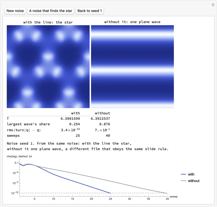
      The published film is labelled r33₁3₂. It is really r3₂*3: nine extra mirrors, hidden in the film. A true r33₁3₂ exists, with . In his engine the delayed lookup did not form it: 0 of 9 from noise, at one setting.

      Try it: press Play and compare the two hands

      Mathematica
      (* The true r33_13_2 film and its mirror image, side by side, with the screw axes its spots circle marked. Solved here by the twisted average from the gyroid formula: a = 1, b = 3.2, Du = 1, Dv = 2.5, box 17.4, N = 36, T = 9.55705; N = 18, 24, 54 give 9.744, 9.624, 9.531. 25 s on the M5. *)
      {handN, handL, handA, handB, handDv} = {36, 17.4, 1., 3.2, 2.5};
      handDt = Min[0.02, 0.15 (handL/handN)^2/handDv];
      handLap[f_] := 2/(3 (handL/handN)^2) ListCorrelate[{{1, 1, 0}, {1, -6, 1}, {0, 1, 1}}, f, {2, 2}];
      handF[q_] := With[{u = q[[1]], v = q[[2]], r = q[[1]]^2 q[[2]]},
         {handLap[u] + handA - (handB + 1) u + r, handDv handLap[v] + handB u - r}];
      handFlow[q0_, t_] := Module[{q = q0, n = Ceiling[t/handDt], h, k1, k2, k3},
         h = t/n;
         Do[k1 = handF[q]; k2 = handF[q + h/2 k1]; k3 = handF[q + h/2 k2];
          q = q + h/6 (k1 + 2 k2 + 2 k3 + handF[q + h k3]), {n}];
         q];
      handOps = Flatten[Table[{m, s[[1]], s[[2]]},
          {m, {{{1, 0}, {0, 1}}, {{-1, 1}, {-1, 0}}, {{0, -1}, {1, -1}}}},
          {s, {{{0, 0}, 0}, {{1/3, 2/3}, 2}, {{2/3, 1/3}, 1}}}], 1];
      handMap[{m_, v_, k_}] := Flatten@Table[With[{g = Mod[m.{x, y} + v handN, handN]}, g[[2]] handN + g[[1]] + 1], {y, 0, handN - 1}, {x, 0, handN - 1}];
      handMaps = {handMap[#], #[[3]] + 1} & /@ handOps;
      handAverage[q_, T_] := Module[{f1 = handFlow[q, T/3], f2, frames, slide},
         f2 = handFlow[f1, T/3];
         frames = Flatten[#, {{1}, {2, 3}}] & /@ {q, f1, f2};
         slide = ArrayReshape[frames[[2, All, handMaps[[3, 1]]]], {2, handN, handN}];
         {ArrayReshape[Mean[frames[[#[[2]], All, #[[1]]]] & /@ handMaps], {2, handN, handN}], slide - q}];
      handK2 = (4 Pi/(Sqrt[3.] handL))^2;
      handHopf = {{handA^2 + handDv handK2, handA^2}, {-(1 + handA^2 + (1 + handDv) handK2), -handA^2 - handDv handK2}};
      handWave = With[{e = Eigensystem[handHopf]}, With[{w = e[[2, First@Ordering[Im[e[[1]]], -1]]]}, w/w[[1]]]];
      handHex = With[{e = Eigensystem[{{handB - 1 - 3 handK2, handA^2}, {-handB, -handA^2 - 3 handDv handK2}}]}, With[{w = e[[2, First@Ordering[Re[e[[1]]], -1]]]}, Re[w/w[[1]]]]];
      handQ = With[{p1 = Table[2. Pi x/handN, {y, 0, handN - 1}, {x, 0, handN - 1}], p2 = Table[2. Pi (y - x)/handN, {y, 0, handN - 1}, {x, 0, handN - 1}], p3 = Table[-2. Pi y/handN, {y, 0, handN - 1}, {x, 0, handN - 1}]},
         {ConstantArray[handA, {handN, handN}], ConstantArray[handB/handA, {handN, handN}]} +
          0.3 Re[Outer[Times, handWave, Exp[I p1] + Exp[I p2] + Exp[I p3]]] +
          0.3 Outer[Times, handHex, Sin[p1 - p2] + Sin[p2 - p3] + Sin[p3 - p1]]];
      {handT, handT0, handSweep, handRes} = {10., 10., 0, 1.};
      Monitor[
        While[handRes > 1*^-10 && handSweep < 300,
         {handNext, handR} = handAverage[handQ, handT];
         handRes = Sqrt[Mean[Flatten[handR^2]]];
         If[handRes > 1*^-10,
          If[handSweep >= 10,
           With[{f = handF[handQ]}, handT = Clip[handT - Clip[3 Total[handR f, 3]/Total[f f, 3], {-0.01, 0.01} handT], {0.7, 1.4} handT0]]];
          handQ = handNext];
         handSweep++],
        Row[{"sweep ", handSweep, "   T = ", handT, "   mismatch ", handRes}]];
      Print["T = ", handT, " after ", handSweep, " sweeps at N = ", handN, "; mismatch ", handRes];
      handFilm = NestList[handFlow[#, handT/48] &, handQ, 47];
      handMirrorIndex = Flatten@Table[Mod[-x, handN] handN + Mod[-y, handN] + 1, {y, 0, handN - 1}, {x, 0, handN - 1}];
      handMirror[u_] := ArrayReshape[Flatten[u][[handMirrorIndex]], {handN, handN}];
      handRange = MinMax[handFilm[[All, 1]]];
      handView = 0.72 handL {-1, 1};
      {handI, handJ} = Transpose[Table[With[{x = handView[[2]] ((c - 1/2)/120 - 1), y = handView[[2]] (1 - (r - 1/2)/120)}, {x/handL + y/(Sqrt[3.] handL), 2 y/(Sqrt[3.] handL)}], {r, 240}, {c, 240}], {2, 3, 1}];
      handImage[u_] := Image[Image[Threaded[{30, 42, 130}/255.] + TensorProduct[Clip[ListInterpolation[ArrayPad[Rescale[u, handRange], {{0, 1}, {0, 1}}, "Periodic"], {{0., 1.}, {0., 1.}},
              PeriodicInterpolation -> True, InterpolationOrder -> 3][handJ, handI], {0., 1.}], {215, 206, 125}/255.]], "Byte"];
      handPlace[{i_, j_}] := handL {i - j/2, j Sqrt[3.]/2};
      handAxes[list_] := Select[Flatten[Table[handPlace[c + {a, b}], {c, list}, {a, -2, 2}, {b, -2, 2}], 2], Max[Abs[#]] < 0.72 handL &];
      handMark[c_, sense_] := {RGBColor[1, 0.69, 0], Disk[c, 0.15], Thick, Arrowheads[0.03],
         Arrow[Table[c + 1.1 {Cos[t], sense Sin[t]}, {t, 0.5, 5.4, 0.05}]]};
      handPanel[u_, title_, axes_, sense_] := Graphics[{
          Inset[handImage[u], {handView[[1]], handView[[1]]}, {Left, Bottom}, 2 handView[[2]] {1, 1}],
          handMark[#, sense] & /@ handAxes[axes]},
         PlotLabel -> title, ImageSize -> 340, PlotRange -> {handView, handView}, PlotRangePadding -> 0];
      handFrames = Row[{
            handPanel[#[[1]], "True film: spots go anticlockwise", {{2/3, 0}, {1/3, 1/3}, {0, 2/3}}, 1],
            handPanel[handMirror[#[[1]]], "Its mirror image: clockwise", {{0, 1/3}, {1/3, 0}, {2/3, 2/3}}, -1]}, Spacer[8]] & /@ handFilm;
      ListAnimate[handFrames, 8]
      

      Download two-hands.wl

      The true film and its mirror image side by side, with the axes its spots circle marked, anticlockwise and clockwise.
      What this draws, in Wolfram 15.0, 00:25

      The reason: the published film is built on three equal waves at , and those always carry mirrors. The gyroid formula, , does not. The hand is the way the spots circle their : only a mirror reverses it.

      The true film, measured: mirror-odd 0.475, and it stays under refinement

      , , , , box side 17.4. Mirror-odd, the smallest rms of the film minus any reflection of it, over twice the pattern's rms: 0.475 with an exact Laplacian, where no mesh direction exists to blame, against for the published film. Its hands are separate films, 0.96 apart. : on this 36 mesh, with an exact Laplacian. Each spot goes round its axis once a period, exactly; the radius runs 1.42 to 2.30, so it is no circle. Stability: unstable, its unison pair a period. His engine's 0 of 9 says little about the film's stability under the lookup: it is one setting, and the 21 of 24 below came from the bare average.

      From noise by the bare average: 21 of 24 starting from the rest state's clock , known from and alone; 1 of 12 started at exactly ; 0 of 24 with the program of section 16, whose free period lets win. From the gyroid formula: 4 of 4, by its author. Source: an independent check of the dynamics, in part2-numbers.json.

      All 116 orbits of the published atlas of films, and all 51 groups

      Atlas. Of 116 published orbits, 52 carry exactly their label and 60 a bigger group that is named right; 1 is one plane wave and 3 are stripes or travelling waves, with a continuous translation. No hidden near-symmetry at any tolerance. Five long-period Ginzburg-Landau orbits read their mirror-image group as the mesh refines: their slow phase rotation changes sign, so none is an example of a hand. Coverage. From noise, on the Brusselator, exactly the group on 19; re-solved at up to three box sizes and on an exact Laplacian, 19 of the 20 first counted survive, the loss a stripe. Carrying the group, possibly with more: 51 of 51 by its author's count, not re-measured. The test that decides: a reading on one mesh passed a film that is mirror-symmetric in the continuum, turned on a smaller cell, so an exact claim needs the waves' own lattice and a search off the mesh. Source: an independent check of the groups, in part2-numbers.json.

      16. Apart from the extension: the simplest versions

      Simplest algorithm: simulate a period, back, average. From noise, with no history and no Newton.

      Try it: run it from noise

      sweep 0 -

      One sweep: frames at , , ; slide the second back one step, the third two; average.

      Mathematica
      (* Noise to the 333 film by simulate, slide back, average: the field after each sweep, then one period, with T and the slide mismatch printed. N = 36, dt = 0.02, T = 6.3901599. 15 s on the M5. *)
      {avgN, avgL, avgA, avgB, avgDt} = {36, 40., 1., 2.3, 0.02};
      avgLap[f_] := 2/(3 (avgL/avgN)^2) ListCorrelate[{{1, 1, 0}, {1, -6, 1}, {0, 1, 1}}, f, {2, 2}];
      avgF[q_] := With[{u = q[[1]], v = q[[2]], r = q[[1]]^2 q[[2]]},
         {avgLap[u] + avgA - (avgB + 1) u + r, avgLap[v] + avgB u - r}];
      avgFlow[q0_, t_] := Module[{q = q0, n = Ceiling[t/avgDt], h, k1, k2, k3},
         h = t/n;
         Do[k1 = avgF[q]; k2 = avgF[q + h/2 k1]; k3 = avgF[q + h/2 k2];
          q = q + h/6 (k1 + 2 k2 + 2 k3 + avgF[q + h k3]), {n}];
         q];
      avgSlide[q_] := RotateLeft[q, {0, avgN/3, 2 avgN/3}];
      avgTurnIndex = Flatten@Table[Mod[x - y, avgN] avgN + Mod[-y, avgN] + 1, {y, 0, avgN - 1}, {x, 0, avgN - 1}];
      avgTurn[q_] := ArrayReshape[Flatten[q, {{1}, {2, 3}}][[All, avgTurnIndex]], {2, avgN, avgN}];
      avgSweep[q_, T_] := Module[{q0 = avgFlow[q, T], f1, f2, r, f},
         f1 = avgFlow[q0, T/3];
         f2 = avgFlow[f1, T/3];
         r = avgSlide[f1] - q0;
         f = avgF[q0];
         {q0, (q0 + avgSlide[f1] + avgSlide[avgSlide[f2]])/3, T - Clip[3 Total[r f, 3]/Total[f f, 3], {-0.1, 0.1}], Sqrt[Mean[Flatten[r^2]]]}];
      SeedRandom[1];
      avgQ = {ConstantArray[avgA, {avgN, avgN}], ConstantArray[avgB/avgA, {avgN, avgN}]} + RandomVariate[NormalDistribution[0, 0.1], {2, avgN, avgN}];
      avgQ = (avgQ + avgTurn[avgQ] + avgTurn[avgTurn[avgQ]])/3;
      {avgT, avgSweeps, avgMismatch, avgFields} = {6.355, 0, 1., {{"noise", avgQ[[1]]}}};
      Monitor[
        While[avgMismatch > 1*^-10 && avgSweeps < 400,
         {avgFirst, avgNext, avgTNext, avgMismatch} = avgSweep[avgQ, avgT];
         avgSweeps++;
         AppendTo[avgFields, {"sweep " <> ToString[avgSweeps], avgFirst[[1]]}];
         If[avgMismatch > 1*^-10, {avgQ, avgT} = {avgNext, avgTNext}]],
        Row[{"sweep ", avgSweeps, "   T = ", avgT, "   mismatch ", avgMismatch}]];
      Print["T = ", avgT, " after ", avgSweeps, " sweeps; slide mismatch ", avgMismatch];
      avgFilm = NestList[avgFlow[#, avgT/48] &, avgFirst, 47];
      avgFields = Join[avgFields, Table[{"one period, frame " <> ToString[j], avgFilm[[j, 1]]}, {j, 48}]];
      avgRange = MinMax[avgFilm[[All, 1]]];
      {avgI, avgJ} = Transpose[Table[With[{x = 32 ((c - 1/2)/120 - 1), y = 11.55 + 32 (1 - (r - 1/2)/120)}, {x/avgL + y/(Sqrt[3.] avgL), 2 y/(Sqrt[3.] avgL)}], {r, 240}, {c, 240}], {2, 3, 1}];
      avgImage[u_] := Image[Image[Threaded[{30, 42, 130}/255.] + TensorProduct[Clip[ListInterpolation[ArrayPad[Rescale[u, avgRange], {{0, 1}, {0, 1}}, "Periodic"], {{0., 1.}, {0., 1.}},
              PeriodicInterpolation -> True, InterpolationOrder -> 3][avgJ, avgI], {0., 1.}], {215, 206, 125}/255.]], "Byte"];
      avgPicture[{label_, u_}] := Graphics[
         Inset[avgImage[u],
          {-32., -20.45}, {Left, Bottom}, {64., 64.}],
         PlotLabel -> label, ImageSize -> 300, PlotRange -> {{-32., 32.}, {-20.45, 43.55}}, PlotRangePadding -> 0];
      avgFrames = avgPicture /@ avgFields;
      ListAnimate[avgFrames, 6]
      

      Download twisted-average.wl

      The field at a late sweep beside a frame of the settled period, both the film.
      What this draws, in Wolfram 15.0, 00:16

      Part 3 takes this program line by line, with a small live diagram for each.

      The program, and the factor per sweep
      unison: closes, sum near 0the film: lines up, stays
      Why it cancels the unison mode: its three frames sit apart, so their average is of it. The film gives three equal arrows.
      Mathematica
      (* Three arrows 1, mu, mu^2 head to tail: why the average over a third of a period cancels the unison mode. The dashed arrow is their sum; (1+mu+mu^2)/3 is the factor one sweep multiplies the mode by. On the M5: under a second to appear, 0.1 s per slider position. *)
      taFactor[taMu_] := (1 + taMu + taMu^2)/3;
      taPicture[taMag_, taDeg_] := With[{taMu = taMag Exp[I taDeg Degree]}, With[{taStops = ReIm /@ Accumulate[{0, 1, taMu, taMu^2}]},
          Graphics[{
            {Thick, Arrowheads[0.05], MapThread[{#1, Arrow[{#2, #3}]} &,
              {{RGBColor[0.19, 0.29, 0.78], RGBColor[0.75, 0.35, 0], RGBColor[0, 0.55, 0.45]}, Most[taStops], Rest[taStops]}]},
            {Dashed, Black, Arrow[{First[taStops], Last[taStops]}]},
            MapThread[Text[#1, Mean[{#2, #3}], {0, -1.6}] &,
             {{"1", "\[Mu]", Superscript["\[Mu]", 2]}, Most[taStops], Rest[taStops]}]},
           PlotRange -> {{-2, 4.2}, {-2.6, 2.6}}, ImageSize -> 440, Axes -> True, Ticks -> None,
           PlotLabel -> Row[{"(1 + \[Mu] + ", Superscript["\[Mu]", 2], ")/3 = ", NumberForm[Chop[N[taFactor[taMu]], 10^-12], {4, 3}],
              ",   size ", NumberForm[Abs[N[taFactor[taMu]]], {4, 3}]}]]]];
      Manipulate[taPicture[taMag, taDeg],
       {{taMag, 1.05, "Size of \[Mu]"}, 0.5, 1.3, 0.001, Appearance -> "Labeled"},
       {{taDeg, 120, "Angle of \[Mu] (degrees)"}, -180, 180, 0.01, Appearance -> "Labeled"},
       Row[{Button["Unison mode: closes", taMag = 1.1608^(1/3.); taDeg = 119.81], Button["The film: lines up", taMag = 1; taDeg = 0],
         Button["Slowest mode", taMag = 0.5235^(1/3.); taDeg = 0]}],
       SaveDefinitions -> True]
      

      Download three-arrows.wl

      Three arrows head to tail, nearly closing, with sliders for the multiplier, three presets and the factor as a number.
      What this draws, in Wolfram 15.0, 00:01

      twisted_average.py, and twisted-average.mjs running here. 300 of 300 seeds by its author; 20 of 20 fresh seeds in the verifier's hands, using no answer: starts at the rest state's clock , known from and . A mode with multiplier per third of a period is multiplied by by the bare average, and by in this file, which runs a free period first: and on the slowest mode. The free period is tuned to this film's weak : it fails on the true film of section 15.

      #!/usr/bin/env python3
      """From white noise to the 333 Brusselator film: simulate, slide back, average.
      
      The film obeys one rule: slide the picture by a third of the box, and it matches
      itself a third of a period later. So take frames a third of a period apart, slide
      them back, and average. What obeys the rule survives, as three copies of one picture.
      Anything ticking in unison is caught at three phases 120 degrees apart, and cancels.
      
          python3 twisted_average.py [seed]        needs only NumPy; about 7 s on one core
      """
      import sys
      
      import numpy as np
      
      N, L = 36, 40.0     # a triangular mesh of N x N nodes, in a repeating box of side L
      a, b = 1.0, 2.3     # the Brusselator's constants; both chemicals diffuse at rate 1
      dt = 0.02           # the longest time step
      
      
      def rate(q):
          """How fast the chemicals q = (u, v) are changing: diffusion plus reaction."""
          u, v = q
          neighbours = [(0, 1), (0, -1), (1, 0), (-1, 0), (1, 1), (-1, -1)]
          laplacian = (sum(np.roll(q, d, (1, 2)) for d in neighbours) - 6 * q) * 2 / (3 * (L / N) ** 2)
          return laplacian + np.array([a - (b + 1) * u + u * u * v, b * u - u * u * v])
      
      
      def simulate(q, t):
          """Run time forward by t (fourth-order Runge-Kutta)."""
          steps = int(np.ceil(t / dt))
          h = t / steps
          for _ in range(steps):
              k1 = rate(q)
              k2 = rate(q + h / 2 * k1)
              k3 = rate(q + h / 2 * k2)
              k4 = rate(q + h * k3)
              q = q + h / 6 * (k1 + 2 * k2 + 2 * k3 + k4)
          return q
      
      
      def slide(q):
          """Slide the picture by a third of the box. On the film this costs T/3 of time."""
          return np.roll(q, (-N // 3, -2 * N // 3), (1, 2))
      
      
      def turn(q):
          """Turn the picture 120 degrees about the origin. On the film this costs no time."""
          y, x = np.indices((N, N))
          return q[:, (x - y) % N, -y % N]
      
      
      def find_film(q, T=6.355, tol=1e-10):
          """Return one frame of the film, its period T, and the number of sweeps it took."""
          q = (q + turn(q) + turn(turn(q))) / 3           # costs no time, so impose it once and it stays
          for sweep in range(1, 400):
              q = simulate(q, T)                          # one free period: what decays, decays
              third = simulate(q, T / 3)
              two_thirds = simulate(third, T / 3)
      
              lag = slide(third) - q                      # zero on the film
              if np.sqrt(np.mean(lag * lag)) < tol:
                  return q, T, sweep
      
              # T is off by 3 x lag / speed. Move it gently, since at first it's all noise.
              speed = rate(q)
              T -= np.clip(3 * np.sum(lag * speed) / np.sum(speed * speed), -0.1, 0.1)
      
              # What obeys the rule survives the average; what ticks in unison cancels.
              q = (q + slide(third) + slide(slide(two_thirds))) / 3
          raise RuntimeError('no convergence')
      
      
      if __name__ == '__main__':
          seed = int(sys.argv[1]) if len(sys.argv) > 1 else 1
          rest = np.array([a, b / a])[:, None, None]
          noise = np.random.default_rng(seed).standard_normal((2, N, N))
          frame, T, sweeps = find_film(rest + 0.1 * noise)
          print(f'seed {seed}: T = {T:.10f} after {sweeps} sweeps (the published film: 6.3901599186)')
      Mathematica
      (* From white noise to the 333 Brusselator film: simulate, slide back, average.
      
         The film obeys one rule: slide the picture by a third of the box, and it matches
         itself a third of a period later. So take frames a third of a period apart, slide
         them back, and average. What obeys the rule survives, as three copies of one picture.
         Anything ticking in unison is caught at three phases 120 degrees apart, and cancels.
      
         Paste into one cell and evaluate. Needs nothing else. About 5 s on an M5. *)
      
      n = 36; box = 40.;   (* a triangular mesh of n x n nodes, in a repeating box of this side *)
      a = 1.; b = 2.3;     (* the Brusselator's constants; both chemicals diffuse at rate 1 *)
      dt = 0.02;           (* the longest time step *)
      
      (* How fast the chemicals q = {u, v} are changing: diffusion plus reaction. *)
      laplacian[f_] := 2/(3 (box/n)^2) ListCorrelate[{{1, 1, 0}, {1, -6, 1}, {0, 1, 1}}, f, {2, 2}];
      rate[{u_, v_}] := {laplacian[u] + a - (b + 1) u + u^2 v, laplacian[v] + b u - u^2 v};
      
      (* Run time forward by t (fourth-order Runge-Kutta). *)
      simulate[q0_, t_] := Module[{q = q0, steps = Ceiling[t/dt], h, k1, k2, k3, k4},
         h = t/steps;
         Do[
          k1 = rate[q];
          k2 = rate[q + h/2 k1];
          k3 = rate[q + h/2 k2];
          k4 = rate[q + h k3];
          q += h/6 (k1 + 2 k2 + 2 k3 + k4),
          {steps}];
         q];
      
      (* Slide the picture by a third of the box. On the film this costs T/3 of time. *)
      slide[q_] := RotateLeft[q, {0, n/3, 2 n/3}];
      
      (* Turn the picture 120 degrees about the origin. On the film this costs no time. *)
      turn[q_] := Table[f[[Mod[x - y, n] + 1, Mod[-y, n] + 1]], {f, q}, {y, 0, n - 1}, {x, 0, n - 1}];
      
      (* One frame of the film, its period T, and the number of sweeps it took. *)
      findFilm[q0_, T0_ : 6.355, tol_ : 1*^-10] := Module[{q, T = T0, third, twoThirds, lag, speed},
         q = (q0 + turn[q0] + turn[turn[q0]])/3;    (* costs no time, so impose it once and it stays *)
         Do[
          q = simulate[q, T];                       (* one free period: what decays, decays *)
          third = simulate[q, T/3];
          twoThirds = simulate[third, T/3];
      
          lag = slide[third] - q;                   (* zero on the film *)
          If[RootMeanSquare[Flatten[lag]] < tol, Return[{q, T, sweep}, Module]];
      
          (* T is off by 3 x lag / speed. Move it gently, since at first it's all noise. *)
          speed = rate[q];
          T -= Clip[3 Total[lag speed, 3]/Total[speed speed, 3], {-0.1, 0.1}];
      
          (* What obeys the rule survives the average; what ticks in unison cancels. *)
          q = (q + slide[third] + slide[slide[twoThirds]])/3,
          {sweep, 399}];
         $Failed];
      
      (* Start from the rest state plus white noise, and find the film. *)
      rest = {ConstantArray[a, {n, n}], ConstantArray[b/a, {n, n}]};
      {frame, T, sweeps} = findFilm[rest + RandomVariate[NormalDistribution[0, 0.1], {2, n, n}]];
      Print["T = ", ToString[NumberForm[T, 11]], " after ", sweeps, " sweeps (the published film: 6.3901599186)"];
      
      (* Play one period of chemical u, on the plane: the mesh's two axes are 120 degrees apart. *)
      film = NestList[simulate[#, T/48] &, frame, 47][[All, 1]];
      range = MinMax[film];
      picture[u_] := Colorize[
         Quiet[    (* Wolfram 15's ImageTransformation trips on the notebook's light/dark background, harmlessly *)
          ImageTransformation[Image[Rescale[Reverse[u], range]],
           {#[[1]] + #[[2]]/Sqrt[3.], 2 #[[2]]/Sqrt[3.]}/box + 0.5/n &, {420, 420},
           DataRange -> {{0, 1}, {0, 1}}, PlotRange -> {{-40., 40.}, {-40., 40.}},
           Padding -> "Periodic", Resampling -> "Bicubic"],
          RemoveAlphaChannel::imginv],
         ColorFunction -> "DeepSeaColors", ColorFunctionScaling -> False];
      ListAnimate[picture /@ film, 12]
      

      Download symmetric-film.wl

      One frame of the film on the plane: triangles of bright spots around dark hexagons.
      What this draws, in Wolfram 15.0, 00:04
      The bake-off: every other algorithm tried
      AlgorithmStartReachCost, right-hand sidesLinesConcepts
      Twisted average: a free period, three frames, slide back, averagenoise300 of 30055,536444
      Same, no free periodnoise50 of 5092,732404
      Published route: envelope, lift, Newton-Krylovnoise20 of 20315,622419
      Newton-Krylov from three wavesseed20 of 2045,803568
      Anderson on the averagenoise20 of 2038,382765
      Recursive projectionnoise20 of 2066,234766
      Delay feedbacknoise20 of 2062,503675
      L-BFGS through the simulatornoise9 of 20257,9571166
      Harmonic balanceseed20 of 207,2211298
      Harmonic balancenoise0 of 20-1298

      Lines count the script alone; the concepts are a judgment. Reach is k of n from the start named. Source: bakeoff.json. The delayed lookup is not a row here: 12 of 12 with no average, and it extends his code.

      Simplest animation: no equation at all.

      Try it: play three films by formula

      Blink, on cells. c*44₂2₁ᵃ

      Three waves. r3₂*3

      Gyroid: six waves, no mirror. r33₁3₂

      Mathematica
      (* Three films by formula, no equation: the blink on cells, three waves, the gyroid slice. One time control, in the phase th: a whole period of the blink and of the three waves is 2 Pi, of the gyroid Pi. On the M5: about 1 s to appear, 0.3 s per position. *)
      (* The blink: (x + y + t) mod 2 on 8 by 8 cells, one step of t every half period. *)
      tfBlink[tfTh_] := Mod[Outer[Plus, Range[8], Range[8]] + Floor[tfTh/Pi], 2];
      (* Both smooth films read X, Y, Z from one plane sliding along the diagonal of the cube. *)
      tfXYZ[tfI_, tfJ_, tfTh_] := {2 Pi tfI - tfTh, 2 Pi (tfJ - tfI) - tfTh, -2 Pi tfJ - tfTh};
      tfThree[{tfX_, tfY_, tfZ_}] := Cos[tfX] + Cos[tfY] + Cos[tfZ];
      tfGyroid[{tfX_, tfY_, tfZ_}] := Sin[tfX] Cos[tfY] + Sin[tfY] Cos[tfZ] + Sin[tfZ] Cos[tfX];
      tfBlue[tfV_] := Blend[{RGBColor[30/255, 42/255, 130/255], RGBColor[64/255, 84/255, 206/255],
          RGBColor[150/255, 170/255, 240/255], RGBColor[245/255, 248/255, 1]}, tfV];
      tfArrays[tfTh_] := With[{tfJ = Transpose[ConstantArray[Subdivide[1.05, -1.05, 199]/(Sqrt[3.]/2), 200]],
          tfXs = ConstantArray[Subdivide[-1.05, 1.05, 199], 200]}, tfXYZ[tfXs + tfJ/2, tfJ, N[tfTh]]];
      tfSmooth[tfLabel_, tfData_] := ArrayPlot[tfData, ColorFunction -> tfBlue, ColorFunctionScaling -> False, Frame -> False,
         ImageSize -> 230, PlotLabel -> tfLabel];
      tfShow[tfTh_] := With[{tfA = tfArrays[tfTh]}, Row[{
           ArrayPlot[tfBlink[tfTh], ColorRules -> {0 -> tfBlue[0], 1 -> tfBlue[1]}, Frame -> False, ImageSize -> 230,
            PlotLabel -> Row[{"Blink, on cells: ", Subscript["c*44", 2], Subsuperscript["2", 1, "a"]}]],
           tfSmooth[Row[{"Three waves: ", Subscript["r3", 2], "*3"}], (tfThree[tfA] + 3/2)/(9/2)],
           tfSmooth[Row[{"Gyroid, no mirror: ", Subscript["r33", 1], Subscript["3", 2]}], (tfGyroid[tfA] + 3/2)/3]}, Spacer[6]]];
      Animate[tfShow[tfTime], {{tfTime, 0.4, "Time (phase)"}, 0, 2 Pi}, AnimationRunning -> False, AnimationRate -> 0.6, SaveDefinitions -> True]
      

      Download three-films.wl

      The blink, three waves and the gyroid slice in a row, under one time control.
      What this draws, in Wolfram 15.0, 00:01
      The ladder of simplest films, and the catches
      FilmGroupWavesCan run backwards
      , read on cellsc*44₂2₁ᵃone bityes
      c*222₁2₁ᵃ3yes
      r3₂*33yes
      , triangular cellsr3₂*3one tritno, on its cells
      c*44₂2₁ᵃ4yes
      c4₃*24yes
      r3₂*34no
      Gyroid slicer33₁3₂6yes

      One or two waves have a continuous translation, so a film needs three. Every three-wave film can be run backwards; a strictly forward formula needs four for one field. The blink's group is true of its cells; as a smooth function its waves collapse, and the smooth film with its group is . is a different group. Source: an independent check of the groups, in part2-numbers.json.

      Simplest law that finds a film: clocks that repel

      Clocks that push away from their neighbours, by : .

      Try it: start 12 by 12 random clocks

      Colour: . 197 of 200 random starts lock into the checkerboard, neighbours half a period apart: the blink, c*44₂2₁ᵃ on the grid.

      Mathematica
      (* Twelve by twelve clocks on a square torus, each pushing away from its four neighbours, from a uniform random start: cos(phase) settling to the blinking checkerboard. 2 s on the M5. *)
      {clockL, clockOmega, clockDt} = {12, 1., 0.1};
      clockF[th_] := clockOmega - Total[Sin[RotateLeft[th, #] - th] & /@ {{0, 1}, {0, -1}, {1, 0}, {-1, 0}}];
      clockStep[th_] := Module[{k1 = clockF[th], k2, k3},
         k2 = clockF[th + clockDt/2 k1];
         k3 = clockF[th + clockDt/2 k2];
         th + clockDt/6 (k1 + 2 k2 + 2 k3 + clockF[th + clockDt k3])];
      clockStagger = Pi Table[x + y, {y, clockL}, {x, clockL}];
      clockOrder[th_] := Abs[Mean[Flatten[Exp[I (th - clockStagger)]]]];
      SeedRandom[7];
      clockTh = RandomReal[{0, 2 Pi}, {clockL, clockL}];
      clockFields = {clockTh};
      clockSteps = 0;
      Monitor[
        While[clockSteps < 10000 && 1 - clockOrder[clockTh] > 1*^-6,
         clockTh = clockStep[clockTh]; clockSteps++;
         If[Mod[clockSteps, 4] == 0, AppendTo[clockFields, clockTh]]];
        clockReached = 1 - clockOrder[clockTh] <= 1*^-6;
        Do[clockTh = clockStep[clockTh]; If[Mod[s, 4] == 0, AppendTo[clockFields, clockTh]], {s, 126}],
        Row[{"time ", clockSteps clockDt, "   order ", clockOrder[clockTh]}]];
      Print[If[clockReached, "Reached the checkerboard at time ", "No checkerboard by time "], clockSteps clockDt, "; order 1 - ", 1 - clockOrder[clockTh]];
      clockColor = Blend[{RGBColor[30/255, 42/255, 130/255], RGBColor[245/255, 248/255, 1]}, #] &;
      clockFrames = MapIndexed[ArrayPlot[(1 + Cos[#1])/2, PlotRange -> {0, 1}, ColorFunction -> clockColor, ColorFunctionScaling -> False, Frame -> False,
           ImageSize -> 300, PlotLabel -> "time " <> ToString[NumberForm[0.4 (First[#2] - 1), {4, 1}]]] &, clockFields];
      ListAnimate[clockFrames, 8]
      

      Download repelling-clocks.wl

      Twelve by twelve clocks locked into the checkerboard, at two moments.
      What this draws, in Wolfram 15.0, 00:02
      Brusselator cells that do this by themselves, and what they are not

      Two or three Brusselator reactors, , , joined by a weak link that carries only , settle from noise into antiphase or a three-phase rotation (15 of 15 and 15 of 15). This is a system of a few coupled cells, not the continuous equation: refine the same torus and no periodic film appears (0 of 8 at each mesh tried). Source: an independent check of the groups, in part2-numbers.json.

      Other routes to the 3D orbifold

      Measured by their author on the array of all frames, not re-run by a verifier. Relax the whole film in a pseudo-time , , with the equation's right-hand side. Every multiplier of the one-third-period map becomes a tower of rates , for each integer , so the growing unison mode comes along: bare transport 0 of 3 from noise (ends uniform). With a low-pass filter in : 10 of 10 from noise. Newton on the array from three waves: 9 of 9 at amplitudes 0.3 to 1.4, about 5 s; least squares falls on the rest state, 0 of 16. Isotropic 3D Gray-Scott keeps r33₁3₂ but obeys a 3D law, not the 2D one. An average over the group of a static 3D pattern reads as a film through a plane sliding along the diagonal, which is the block of section 9.

      The orbifold of r33₁3₂, in plain words
      • Three turns about three axes. Three turns about the first advance one period, about the second two, about the third none, and all three in a row advance one.
      • Only one line in the whole crystal has a real symmetry point: the pure axis. A screw axis is a marked place in the film, but nothing is special there in the crystal.
      • Forget the marking and the space is a sphere carried once around a circle. The marking is a single loop, one period long, that takes three turns of the one-third-period clock to close, with a wedge around it instead of .
      • A slice folds into a triangular pillow. Advance one third of a period and the pillow has turned about its front and back.
      • Follow one point of the plane through time: a generic one repeats after , one on a screw axis after .
      • The cost rule. The costs around the three axes must add to a whole number of periods; otherwise time would not be consistent around the crystal. Here . Conway and coauthors state it as a homomorphism, modulo the kernel (On three-dimensional space groups, section 3.4).
      • With the mirrors of r3₂*3 the slice folds into a solid triangle instead of a pillow: a ring-shaped solid whose skin is a mirror, half the volume.

      Derived and checked here in exact arithmetic; the sphere and the ring were found in no published table. Source: an independent check of the geometry, in part2-numbers.json.

      Part 3

      The program of section 16, find_film, one line at a time: what each line does, and why it is there.

      17. The whole program, stepped

      What: from noise, one at a time, until a frame slid by a third of the box matches the frame a third of a period earlier.

      Why: that match is the rule the film obeys, so the program stops when the rule holds. Every line below has its own card: tap a line to go to it.

      What one sweep costs, line by line

      Almost all of it is simulation. Rate calls are per sweep at (the film's true period) with , seconds per sweep are one NumPy core (find-film-runs.json, block R15).

      Linerate callsSeconds
      q = simulate(q, T)12800.142
      third = simulate(q, T / 3)4280.047
      two_thirds = simulate(third, T / 3)4280.047
      speed = rate(q)1
      lag = ..., the stop test, T -= ..., the average0each at most

      So a sweep simulates of time. The turn line runs once and costs s.

      What a whole run does, over 200 seeds

      Seeds 1-200, noise amplitude : the film 200 of 200, in 22 to 29 sweeps, median 26, or 43.3 periods of simulated time. The field's spread settles by sweep 7 (median), settles to within by sweep 7, and rms(lag) then falls faster than it will end up, as quicker modes die: 0.22 to 0.40 a sweep at sweeps 8 to 12 (seeds 1 to 120). From about sweep 15 it holds at 0.4288. That number, and a constant read from the run, set the sweep count (the card on both lines together).

      Where the run lands on the loop depends on the seed, and nothing else does: the frame differs, does not (the card on return).

      The cost of a run: 55519 rate calls (median), 7.6 s on one NumPy core. Source: find-film-runs.json, block R1: a separate timing from the table above, block R15, so the two need not multiply out.

      This is the program itself, not a cartoon

      Each button runs the real lines, in the JavaScript port this page already uses (twisted-average.mjs), and To the end takes the same sweeps as twisted_average.py. The listing above is cut from that file when the page is built, so it cannot drift from it.

      Seed 1 here is the very draw of python3 twisted_average.py 1, carried as data, since a browser cannot draw NumPy's generator: it lands in 25 sweeps at , as the Python does (find-film-extra-lab.json). A test compares the two sweep by sweep. They part only at round-off, because the two languages add the six neighbours in a different order. New noise draws from a small generator in this page, the same bell curve but not NumPy's draw for that seed.

      The colours of q, third and two_thirds stretch to their shared range at each step, stated under the panes: at first the field is nearly flat and on the film's range it would look blank. lag and speed show only, and each has its own scale, also stated.

      Mathematica
      (* The whole program, one line at a time. Evaluating this runs find_film from noise and records every line; the controls step through that record with the line that ran lit, and show q, third, twoThirds, lag, speed and rms(lag). About 2 s on an M5; New noise about 2 s more. Noise comes from Wolfram's generator, not NumPy's. *)
      n = 36; box = 40.;   (* a triangular mesh of n x n nodes, in a repeating box of this side *)
      a = 1.; b = 2.3;     (* the Brusselator's constants; both chemicals diffuse at rate 1 *)
      dt = 0.02;           (* the longest time step *)
      
      (* How fast the chemicals q = {u, v} are changing: diffusion plus reaction. *)
      laplacian[f_] := 2/(3 (box/n)^2) ListCorrelate[{{1, 1, 0}, {1, -6, 1}, {0, 1, 1}}, f, {2, 2}];
      rate[{u_, v_}] := {laplacian[u] + a - (b + 1) u + u^2 v, laplacian[v] + b u - u^2 v};
      
      (* Run time forward by t (fourth-order Runge-Kutta). *)
      simulate[q0_, t_] := Module[{q = q0, steps = Ceiling[t/dt], h, k1, k2, k3, k4},
         h = t/steps;
         Do[
          k1 = rate[q];
          k2 = rate[q + h/2 k1];
          k3 = rate[q + h/2 k2];
          k4 = rate[q + h k3];
          q += h/6 (k1 + 2 k2 + 2 k3 + k4),
          {steps}];
         q];
      
      (* Slide the picture by a third of the box. On the film this costs T/3 of time. *)
      slide[q_] := RotateLeft[q, {0, n/3, 2 n/3}];
      
      (* Turn the picture 120 degrees about the origin. On the film this costs no time. *)
      turn[q_] := Table[f[[Mod[x - y, n] + 1, Mod[-y, n] + 1]], {f, q}, {y, 0, n - 1}, {x, 0, n - 1}];
      
      (* Start from the rest state plus white noise, and find the film. *)
      rest = {ConstantArray[a, {n, n}], ConstantArray[b/a, {n, n}]};
      noise[s_, amp_ : 0.1] := (SeedRandom[s]; rest + RandomVariate[NormalDistribution[0, amp], {2, n, n}]);
      
      (* Four points a mesh step, linear on the mesh's own triangles, as the page paints: a turned field then draws as the turned picture. *)
      meshTent = Table[Max[0., 1. - Max[Abs[i], Abs[j], Abs[i - j]]/4.], {j, -3, 3}, {i, -3, 3}];
      meshFine[f_] := ListCorrelate[meshTent, KroneckerProduct[f, Normal[SparseArray[{{1, 1} -> 1.}, {4, 4}]]], {4, 4}];
      
      (* A field on the plane, as a picture: the mesh's two axes are 120 degrees apart. Blue is lo, white is hi. *)
      picture[u_, {lo_, hi_}, size_ : 240] := Colorize[
         Quiet[    (* Wolfram 15's ImageTransformation trips on the notebook's light/dark background, harmlessly *)
          ImageTransformation[Image[Rescale[Reverse[meshFine[u]], {lo, hi}]],
           {#[[1]] + #[[2]]/Sqrt[3.], 2 #[[2]]/Sqrt[3.]}/box + 0.5/(4 n) &, {size, size},
           DataRange -> {{0, 1}, {0, 1}}, PlotRange -> {{-40., 40.}, {-40., 40.}},
           Padding -> "Periodic", Resampling -> "Linear"],
          RemoveAlphaChannel::imginv],
         ColorFunction -> (Blend[{RGBColor[0.118, 0.165, 0.51], RGBColor[0.251, 0.329, 0.808], RGBColor[0.588, 0.667, 0.941], RGBColor[0.961, 0.973, 1.]}, #] &), ColorFunctionScaling -> False];
      
      (* find_film's own lines, with a mark after each: the listing line, what it did, and the field it wrote. *)
      stRecord[s_] := Module[{q0 = noise[s], q, T = 6.355, tol = 1*^-10, third, twoThirds, lag, speed, sweepNo = 0, lags = {}, frames = {}, at = <||>, rows = {}, mark},
         mark[line_, say_, pane_ : None, f_ : {}] := (
           If[pane =!= None, AppendTo[frames, f[[1]]]; at[pane] = Length[frames]];
           AppendTo[rows, <|"line" -> line, "say" -> say, "pane" -> pane, "sweep" -> sweepNo, "T" -> T, "lags" -> lags, "at" -> at|>]);
         q = q0; mark[1, "The input: q is the rest state plus white noise, T is 6.355.", "q", q];
         q = (q0 + turn[q0] + turn[turn[q0]])/3; mark[2, Row[{"Averaged with its two turns: rms(turn[q] - q) is now ", ScientificForm[RootMeanSquare[Flatten[turn[q] - q]], 2], "."}], "q", q];
         Do[
          sweepNo = sweep; mark[3, Row[{"Sweep ", sweep, " begins."}]];
          q = simulate[q, T]; mark[4, Row[{"One free period of ", NumberForm[T, {5, 4}], "."}], "q", q];
          third = simulate[q, T/3]; mark[5, "q run on by T/3.", "third", third];
          twoThirds = simulate[third, T/3]; mark[6, "Run on by another T/3.", "twoThirds", twoThirds];
          lag = slide[third] - q; AppendTo[lags, RootMeanSquare[Flatten[lag]]]; mark[8, "Slide third back by a third of the box and subtract q.", "lag", lag];
          If[Last[lags] < tol, mark[9, Row[{"rms(lag) = ", ScientificForm[Last[lags], 2], " is below 1e-10: stop. Returned T = ", NumberForm[T, 11], " after ", sweep, " sweeps."}]]; Return[{frames, rows}, Module]];
          mark[9, Row[{"rms(lag) = ", ScientificForm[Last[lags], 2], " is above 1e-10: go on."}]];
          speed = rate[q]; mark[12, "speed is the field's rate of change at q.", "speed", speed];
          T -= Clip[3 Total[lag speed, 3]/Total[speed speed, 3], {-0.1, 0.1}]; mark[13, Row[{"T moves to ", NumberForm[T, {5, 4}], "."}]];
          q = (q + slide[third] + slide[slide[twoThirds]])/3; mark[16, "The three frames, slid back onto q and averaged: this is the next start.", "q", q],
          {sweep, 399}];
         {frames, rows}];
      stRun[s_] := stRun[s] = stRecord[s];
      stRun[1];
      
      (* The listing as it runs: the core's findFilm, line for line. *)
      stListing = {"findFilm[q0_, T0_ : 6.355, tol_ : 1*^-10] := Module[{q, T = T0, third, twoThirds, lag, speed},",
         "   q = (q0 + turn[q0] + turn[turn[q0]])/3;    (* costs no time, so impose it once and it stays *)", "   Do[",
         "    q = simulate[q, T];                       (* one free period: what decays, decays *)", "    third = simulate[q, T/3];", "    twoThirds = simulate[third, T/3];", "",
         "    lag = slide[third] - q;                   (* zero on the film *)", "    If[RootMeanSquare[Flatten[lag]] < tol, Return[{q, T, sweep}, Module]];", "",
         "    (* T is off by 3 x lag / speed. Move it gently, since at first it's all noise. *)", "    speed = rate[q];", "    T -= Clip[3 Total[lag speed, 3]/Total[speed speed, 3], {-0.1, 0.1}];", "",
         "    (* What obeys the rule survives the average; what ticks in unison cancels. *)", "    q = (q + slide[third] + slide[slide[twoThirds]])/3,", "    {sweep, 399}];", "   $Failed];"};
      
      (* |u| on the plane, black is zero, white is hi: the geometry of picture. *)
      stSize[f_, hi_] := Quiet[ImageTransformation[Image[Clip[Abs[Reverse[meshFine[f]]]/hi, {0, 1}]], {#[[1]] + #[[2]]/Sqrt[3.], 2 #[[2]]/Sqrt[3.]}/box + 0.5/(4 n) &, {300, 300},
          DataRange -> {{0, 1}, {0, 1}}, PlotRange -> {{-40., 40.}, {-40., 40.}}, Padding -> "Periodic", Resampling -> "Linear"], RemoveAlphaChannel::imginv];
      
      (* One step of the record: the listing with its line lit, the five fields (orange frame: this line wrote it; grey: not written yet), and rms(lag) so far. *)
      stView[s_, k_] := Module[{frames, r, field, lo, hi, pane},
         {frames, r} = {stRun[s][[1]], stRun[s][[2, k]]};
         field[name_] := If[KeyExistsQ[r["at"], name], frames[[r["at", name]]], None];
         {lo, hi} = With[{m = MinMax[DeleteCases[field /@ {"q", "third", "twoThirds"}, None]]}, Mean[m] + {-1, 1} Max[0.02, m[[2]] - m[[1]]]/2];
         pane[name_, draw_] := Labeled[Framed[Image[If[field[name] === None, ConstantImage[GrayLevel[0.9], {300, 300}], draw[field[name]]], ImageSize -> 150],
             FrameMargins -> 0, FrameStyle -> Directive[Thickness[3], If[r["pane"] === name, Orange, White]]], Style[name, 12, FontFamily -> "Courier"], Top];
         Column[{
           Column[MapIndexed[Item[Style[If[#1 === "", " ", #1], 11, FontFamily -> "Courier"], Background -> If[First[#2] === r["line"], LightBlue, None]] &, stListing], Spacings -> 0, Alignment -> Left],
           Row[{"sweep ", r["sweep"], "     T ", NumberForm[r["T"], {5, 4}], "     rms(lag) ", If[r["lags"] === {}, "-", ScientificForm[Last[r["lags"]], 2]], "     noise seed ", s}],
           r["say"],
           Grid[{Join[pane[#, picture[#, {lo, hi}, 300] &] & /@ {"q", "third", "twoThirds"}, pane[#, stSize[#, Max[Abs[#]]] &] & /@ {"lag", "speed"}]}, Spacings -> 0.3],
           Row[{"Colour: u from ", NumberForm[lo, {4, 3}], " to ", NumberForm[hi, {4, 3}], ". lag and speed show |u|, each on its own scale."}],
           ListLogPlot[If[r["lags"] === {}, {{1, 1}}, r["lags"]], Joined -> True, PlotMarkers -> {Automatic, 5}, PlotStyle -> If[r["lags"] === {}, Opacity[0], Automatic],
            PlotRange -> {{1, Max[30, Length[r["lags"]]]}, {1*^-11, 1}}, GridLines -> {{Max[1, r["sweep"]]}, None}, AxesLabel -> {"sweep", "rms(lag)"}, ImageSize -> 760, AspectRatio -> 1/5,
            Epilog -> {Dashed, Gray, Line[{{1, Log[1*^-10]}, {Max[30, Length[r["lags"]]], Log[1*^-10]}}], Text["tol", {3, Log[1*^-10]}, {0, -1}]}]}, Spacings -> 1]];
      
      Manipulate[
       stView[seed, step],
       {{seed, 1}, ControlType -> None},
       {{step, 1}, ControlType -> None},
       Dynamic[Row[{"Step through the run  ", Manipulator[Dynamic[step], {1, Length[stRun[seed][[2]]], 1}, ImageSize -> 400], "  ", Dynamic[step], " of ", Length[stRun[seed][[2]]]}]],
       Row[{
         Button["Next line", step = Min[step + 1, Length[stRun[seed][[2]]]]],
         Button["Next sweep", step = First[Select[Range[step + 1, Length[stRun[seed][[2]]]], stRun[seed][[2, #, "line"]] === 16 &], Length[stRun[seed][[2]]]]],
         Button["To the end", step = Length[stRun[seed][[2]]]],
         Button["New noise", stRun[seed + 1]; step = 1; seed = seed + 1, Method -> "Queued"]}, " "],
       SaveDefinitions -> True]
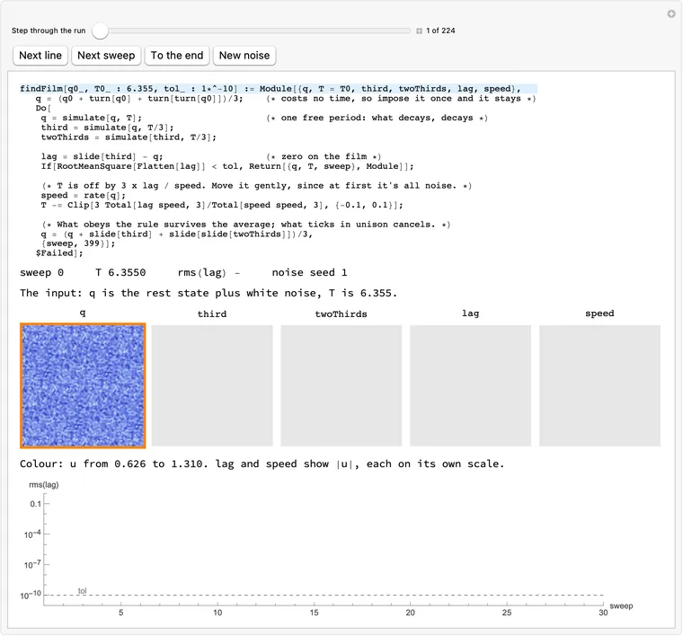
      

      Download ff-step.wl

      The listing of findFilm with the line that ran lit, above the five fields q, third, twoThirds, lag and speed and a log chart of rms(lag) falling to the dashed tolerance.
      What this draws, in Wolfram 15.0, 00:02

      18. What comes out, and what goes in

      """Return one frame of the film, its period T, and the number of sweeps it took."""

      What: the answer is small: one and one number, the period . Everything else in the follows by running time forward from that frame.

      Why: the film is a closed loop among all possible fields, so the program only has to find one point on it and the time once round, not a whole movie.

      Try it: move time forward and watch the loop close

      , made by simulate

      where that is on the

      ()

      Many cards below measure against the , and its period .

      What comes back, exactly, and how closely it closes

      Three things come back. q, 2592 numbers, : the frame after the sweep's free period, not the average (the card on return says why). T, the value that frame was tested with. And sweep, the count.

      "Closes" is a matter of degree, and each degree has a cause. Rms of the field after one period, minus the frame:

      FrameOne simulate(q, T)Three simulate(q, T / 3)
      The exact frame of the page's data
      The frame seed 1 returned, off by

      The exact frame's two columns differ only because a whole period takes 320 Runge-Kutta steps and three thirds take : two slightly different maps (the card on the stop test). The returned frame's error is the run's own: it stopped when rms(lag) fell under , and its true rms distance to the film is to over seeds 5001-5400. Sources: find-film-extra-cardsA.json, block frame; find-film-modes.json, block m1_exact_frame.

      "Everything else follows": how far that is true

      In principle only. A frame returned by the program cannot simply be run for ever. Its error grows 1.152 per period, the film is half gone after 172 to 178 periods (seeds 1-10), and it ends as a nearly uniform field (the card on what the frame cannot do). So a player simulates one period once and loops the stored frames.

      Fewer frames than it looks. Since the film obeys the slide rule, is slid by a third of the box. A player of 48 frames per period needs to compute only 16 of them, and the rest are array shifts.

      The distance curve above has no dip at . At the field is 0.662 from the first frame, nowhere near it, though it is the same picture slid. Only the whole period brings the field itself back. The largest distance is 0.863 and the spread over the mesh is 0.292 for and 0.458 for ; rms here is over both chemicals.

      The picture of the loop is a flattening. The two directions hold 46.7% and 46.7% of the film's variance about its mean. The loop is a rounded triangle, radius 18.4 to 25.3 in these units, with three lobes because the slide turns this plane by exactly each . "One point on it" is also not any point: a run mostly lands near one instant, for a reason the card on return measures.

      Mathematica
      (* The answer is one frame and one number. This finds them from noise, then runs time forward from that frame: the field at time t, where it is on the closed loop, and its rms distance from the first frame, which comes back to almost nothing at one period. About 2 s on an M5. Noise comes from Wolfram's generator; the frame is the one this run returned, not the page's Newton-solved one. *)
      n = 36; box = 40.;   (* a triangular mesh of n x n nodes, in a repeating box of this side *)
      a = 1.; b = 2.3;     (* the Brusselator's constants; both chemicals diffuse at rate 1 *)
      dt = 0.02;           (* the longest time step *)
      
      (* How fast the chemicals q = {u, v} are changing: diffusion plus reaction. *)
      laplacian[f_] := 2/(3 (box/n)^2) ListCorrelate[{{1, 1, 0}, {1, -6, 1}, {0, 1, 1}}, f, {2, 2}];
      rate[{u_, v_}] := {laplacian[u] + a - (b + 1) u + u^2 v, laplacian[v] + b u - u^2 v};
      
      (* Run time forward by t (fourth-order Runge-Kutta). *)
      simulate[q0_, t_] := Module[{q = q0, steps = Ceiling[t/dt], h, k1, k2, k3, k4},
         h = t/steps;
         Do[
          k1 = rate[q];
          k2 = rate[q + h/2 k1];
          k3 = rate[q + h/2 k2];
          k4 = rate[q + h k3];
          q += h/6 (k1 + 2 k2 + 2 k3 + k4),
          {steps}];
         q];
      
      (* Slide the picture by a third of the box. On the film this costs T/3 of time. *)
      slide[q_] := RotateLeft[q, {0, n/3, 2 n/3}];
      
      (* Turn the picture 120 degrees about the origin. On the film this costs no time. *)
      turn[q_] := Table[f[[Mod[x - y, n] + 1, Mod[-y, n] + 1]], {f, q}, {y, 0, n - 1}, {x, 0, n - 1}];
      
      (* One frame of the film, its period T, and the number of sweeps it took. *)
      findFilm[q0_, T0_ : 6.355, tol_ : 1*^-10] := Module[{q, T = T0, third, twoThirds, lag, speed},
         q = (q0 + turn[q0] + turn[turn[q0]])/3;    (* costs no time, so impose it once and it stays *)
         Do[
          q = simulate[q, T];                       (* one free period: what decays, decays *)
          third = simulate[q, T/3];
          twoThirds = simulate[third, T/3];
      
          lag = slide[third] - q;                   (* zero on the film *)
          If[RootMeanSquare[Flatten[lag]] < tol, Return[{q, T, sweep}, Module]];
      
          (* T is off by 3 x lag / speed. Move it gently, since at first it's all noise. *)
          speed = rate[q];
          T -= Clip[3 Total[lag speed, 3]/Total[speed speed, 3], {-0.1, 0.1}];
      
          (* What obeys the rule survives the average; what ticks in unison cancels. *)
          q = (q + slide[third] + slide[slide[twoThirds]])/3,
          {sweep, 399}];
         $Failed];
      
      (* Start from the rest state plus white noise, and find the film. *)
      rest = {ConstantArray[a, {n, n}], ConstantArray[b/a, {n, n}]};
      noise[s_, amp_ : 0.1] := (SeedRandom[s]; rest + RandomVariate[NormalDistribution[0, amp], {2, n, n}]);
      
      (* Four points a mesh step, linear on the mesh's own triangles, as the page paints: a turned field then draws as the turned picture. *)
      meshTent = Table[Max[0., 1. - Max[Abs[i], Abs[j], Abs[i - j]]/4.], {j, -3, 3}, {i, -3, 3}];
      meshFine[f_] := ListCorrelate[meshTent, KroneckerProduct[f, Normal[SparseArray[{{1, 1} -> 1.}, {4, 4}]]], {4, 4}];
      
      (* A field on the plane, as a picture: the mesh's two axes are 120 degrees apart. Blue is lo, white is hi. *)
      picture[u_, {lo_, hi_}, size_ : 240] := Colorize[
         Quiet[    (* Wolfram 15's ImageTransformation trips on the notebook's light/dark background, harmlessly *)
          ImageTransformation[Image[Rescale[Reverse[meshFine[u]], {lo, hi}]],
           {#[[1]] + #[[2]]/Sqrt[3.], 2 #[[2]]/Sqrt[3.]}/box + 0.5/(4 n) &, {size, size},
           DataRange -> {{0, 1}, {0, 1}}, PlotRange -> {{-40., 40.}, {-40., 40.}},
           Padding -> "Periodic", Resampling -> "Linear"],
          RemoveAlphaChannel::imginv],
         ColorFunction -> (Blend[{RGBColor[0.118, 0.165, 0.51], RGBColor[0.251, 0.329, 0.808], RGBColor[0.588, 0.667, 0.941], RGBColor[0.961, 0.973, 1.]}, #] &), ColorFunctionScaling -> False];
      
      {frFrame, frT, frSweeps} = findFilm[noise[1]];
      
      (* Everything else follows by running time forward: 48 steps round the loop, and one whole simulate[q, T] for the end. *)
      frFilm = NestList[simulate[#, frT/48] &, frFrame, 47];
      frEnd = simulate[frFrame, frT];
      frField[j_] := If[j == 48, frEnd, frFilm[[j + 1]]];
      frDistance = Table[RootMeanSquare[Flatten[frField[j] - frFrame]], {j, 0, 48}];
      
      (* The loop flattened onto the two directions in which the film's frames differ most (its first two principal components). *)
      frMean = Mean[Flatten /@ frFilm];
      frAxes = Transpose[Take[SingularValueDecomposition[(Flatten[#] - frMean) & /@ frFilm, 2][[3]], All, 2]];
      frPlane[q_] := frAxes . (Flatten[q] - frMean);
      frLoop = frPlane /@ frFilm;
      frRange = MinMax[frFilm[[All, 1]]];
      
      frView[j_] := Column[{
          Row[{
            Labeled[Image[picture[frField[j][[1]], frRange, 480], ImageSize -> 300], "q(t), made by simulate", Top],
            Labeled[Graphics[{
               {GrayLevel[0.7], Thick, Line[Append[frLoop, First[frLoop]]]},
               {RGBColor[0.2, 0.3, 0.8], Thick, Line[Take[Append[frLoop, First[frLoop]], j + 1]]},
               {Black, PointSize[0.018], Point[First[frLoop]], Text["q", First[frLoop], {-2, 0}]},
               {Black, Thick, Line[frPlane[rest] + # & /@ {{-1, 0}, {1, 0}}], Line[frPlane[rest] + # & /@ {{0, -1}, {0, 1}}]},
               {Orange, PointSize[0.03], Point[Append[frLoop, First[frLoop]][[j + 1]]]}},
              ImageSize -> 300, PlotRange -> All, PlotRangePadding -> Scaled[0.05]], "where that is on the loop; the cross is the rest state", Top]}, "   "],
          ListLinePlot[Transpose[{Range[0, 48]/48. frT, frDistance}], PlotRange -> {{0, frT}, {0, 1}}, AxesLabel -> {"time t since the frame", "rms(q(t) - q)"},
           GridLines -> {{j/48. frT}, None}, GridLinesStyle -> Orange, Epilog -> {Orange, PointSize[0.012], Point[{j/48. frT, frDistance[[j + 1]]}]}, ImageSize -> 620, AspectRatio -> 1/4],
          Row[{"t = ", If[j == 48, Row[{NumberForm[frT, 8], ", one period"}], NumberForm[j/48. frT, {4, 3}]], "     rms(q(t) - q) = ", ScientificForm[frDistance[[j + 1]], 3]}],
          Which[j == 0, "At t = 0: the frame itself.",
           j == 48, Row[{"One whole period on: the same frame, to ", ScientificForm[frDistance[[49]], 2], ". Nothing else had to be stored."}],
           True, "A frame the program never stored: simulate made it from q."]}, Spacings -> 1];
      
      Manipulate[frView[j], {{j, 12, "Time, in 48ths of a period"}, 0, 48, 1, Appearance -> "Labeled"}, SaveDefinitions -> True]
      

      Download ff-frame.wl

      The field at a time slider's position, beside the closed rounded-triangle loop with an orange dot on it, above the rms distance from the first frame, which comes back to almost nothing at one period.
      What this draws, in Wolfram 15.0, 00:02
      def find_film(q, T=6.355, tol=1e-10):

      What: q is the field to start from. The program's last lines call it with of size around the .

      Why: noise holds no pattern, so no picture of the answer goes in: the film that comes out is what the program's rule selects. Its size hardly matters: every seed reaches the film from to 4.

      Try it: change the size of the noise, then press Run

      the noise that goes in

      where it lands

      reach the film, measured sweeps

      Seed 1 at size , as the program is called: this noise went in, and this frame came out 25 sweeps later.

      Both panes: , colour from to . The chart is the measured table below; Run is one live run.

      Why the size hardly matters: each factor of 10 costs about 2.3 sweeps

      Near the rest state the three waves that make the film are multiplied by 2.7549 each sweep (measured on single waves; the card on why three waves). So a noise times smaller needs sweeps more to reach the same size.

      Measured, median sweeps over seeds 1-20: 38 at , 33 at , 31 at , 29 at , 26 at , and 25 at , where it can get no faster, since the field is large from the start.

      A test of that reason, which it first failed. At the law predicts about 42.5 sweeps, two decades on from , but the measured median is 58.5 (seeds 1-20; the readout above is a second table, seeds 10001-10100, and reads 51). So there was something else: the field must grow ten million times, and the round-off that breaks the turn symmetry grows with it (the card on why it stays). The run then has to shed that through modes the first line had removed, the slowest at 0.9557 a sweep. Imposing the turn after every sweep removes the leak: the same three seeds take 55, 66, 42 sweeps as written and 42, 43, 42 with it, as the law says (find-film-extra-cardsA.json, block tiny_noise; numpy seeds 1 to 3).

      Where it fails, at each end, and how: the table
      Noise sizeSeedsReach the filmMedian sweepsThe rest
      1-200 of 201flat, returned, no error
      10001-101000 of 1001flat, returned, no error
      10001-1010053 of 10047 flat
      10001-10100100 of 100
      1-2020 of 2038
      5001-5400400 of 40026
      10201-1024040 of 4025
      10201-1024039 of 40261 blow up
      10201-102408 of 4025.532 blow up
      10201-102400 of 4040 blow up

      The bottom is a false positive of the stop test. A tiny field has a tiny lag, about 0.323 of the noise's size at sweep 1, so the test passes before anything has grown, and the program returns a nearly flat field with no error. A field exactly at rest does the same. It ends near because the lag dips at sweeps 2 and 3 to as little as of the noise's size, and is about that (find-film-runs.json, block R10b; the card on the stop test).

      The top is not the raise. The numbers go NaN, and the Python dies with ValueError: cannot convert float NaN to integer where int(np.ceil(t / dt)) meets it, not with RuntimeError (block R10). The run on this page stops at the same place and reports it.

      What "no answer goes in" leaves out, and what noise this is

      The picture stays out, not the structure. The slide's vector, the turn and the first guess of are all written into the program: they say which crystal to look for, and a different slide finds a different film (the card on slide). What the noise leaves free is only where the pattern starts. Three things about the input: it carries some of every wave, so the waves that grow have something to grow from; it has no symmetry, so the next line must supply it; and at size it is small enough that the first free period behaves almost linearly, apart from the mean.

      What happens to it next. The turn line keeps a third of its power (the card on the first line), and the first free period cuts what lies off the film's plane to 0.0139 from 0.0595 (the card on the free period).

      The draw. The program uses np.random.default_rng(seed).standard_normal((2, N, N)): independent standard normals, the same for both chemicals. No other law was tried. Seed 1 on this page is numpy's own draw, carried as data; New noise draws from a small generator in this page, the same law, so a table row is a statement about the law and not about your seed.

      Mathematica
      (* The argument q: white noise around the rest state. A slider for its size over 15 decades, the noise that goes in, where it lands, and how often the program reaches the film at that size. Run really runs the program on this noise, typically 2 s (up to a minute at the sizes that blow up). About 2 s on an M5 to start. Noise comes from Wolfram's generator, so one run need not match the table. *)
      n = 36; box = 40.;   (* a triangular mesh of n x n nodes, in a repeating box of this side *)
      a = 1.; b = 2.3;     (* the Brusselator's constants; both chemicals diffuse at rate 1 *)
      dt = 0.02;           (* the longest time step *)
      
      (* How fast the chemicals q = {u, v} are changing: diffusion plus reaction. *)
      laplacian[f_] := 2/(3 (box/n)^2) ListCorrelate[{{1, 1, 0}, {1, -6, 1}, {0, 1, 1}}, f, {2, 2}];
      rate[{u_, v_}] := {laplacian[u] + a - (b + 1) u + u^2 v, laplacian[v] + b u - u^2 v};
      
      (* Run time forward by t (fourth-order Runge-Kutta). *)
      simulate[q0_, t_] := Module[{q = q0, steps = Ceiling[t/dt], h, k1, k2, k3, k4},
         h = t/steps;
         Do[
          k1 = rate[q];
          k2 = rate[q + h/2 k1];
          k3 = rate[q + h/2 k2];
          k4 = rate[q + h k3];
          q += h/6 (k1 + 2 k2 + 2 k3 + k4),
          {steps}];
         q];
      
      (* Slide the picture by a third of the box. On the film this costs T/3 of time. *)
      slide[q_] := RotateLeft[q, {0, n/3, 2 n/3}];
      
      (* Turn the picture 120 degrees about the origin. On the film this costs no time. *)
      turn[q_] := Table[f[[Mod[x - y, n] + 1, Mod[-y, n] + 1]], {f, q}, {y, 0, n - 1}, {x, 0, n - 1}];
      
      (* One frame of the film, its period T, and the number of sweeps it took. *)
      findFilm[q0_, T0_ : 6.355, tol_ : 1*^-10] := Module[{q, T = T0, third, twoThirds, lag, speed},
         q = (q0 + turn[q0] + turn[turn[q0]])/3;    (* costs no time, so impose it once and it stays *)
         Do[
          q = simulate[q, T];                       (* one free period: what decays, decays *)
          third = simulate[q, T/3];
          twoThirds = simulate[third, T/3];
      
          lag = slide[third] - q;                   (* zero on the film *)
          If[RootMeanSquare[Flatten[lag]] < tol, Return[{q, T, sweep}, Module]];
      
          (* T is off by 3 x lag / speed. Move it gently, since at first it's all noise. *)
          speed = rate[q];
          T -= Clip[3 Total[lag speed, 3]/Total[speed speed, 3], {-0.1, 0.1}];
      
          (* What obeys the rule survives the average; what ticks in unison cancels. *)
          q = (q + slide[third] + slide[slide[twoThirds]])/3,
          {sweep, 399}];
         $Failed];
      
      (* Start from the rest state plus white noise, and find the film. *)
      rest = {ConstantArray[a, {n, n}], ConstantArray[b/a, {n, n}]};
      noise[s_, amp_ : 0.1] := (SeedRandom[s]; rest + RandomVariate[NormalDistribution[0, amp], {2, n, n}]);
      
      (* Four points a mesh step, linear on the mesh's own triangles, as the page paints: a turned field then draws as the turned picture. *)
      meshTent = Table[Max[0., 1. - Max[Abs[i], Abs[j], Abs[i - j]]/4.], {j, -3, 3}, {i, -3, 3}];
      meshFine[f_] := ListCorrelate[meshTent, KroneckerProduct[f, Normal[SparseArray[{{1, 1} -> 1.}, {4, 4}]]], {4, 4}];
      
      (* A field on the plane, as a picture: the mesh's two axes are 120 degrees apart. Blue is lo, white is hi. *)
      picture[u_, {lo_, hi_}, size_ : 240] := Colorize[
         Quiet[    (* Wolfram 15's ImageTransformation trips on the notebook's light/dark background, harmlessly *)
          ImageTransformation[Image[Rescale[Reverse[meshFine[u]], {lo, hi}]],
           {#[[1]] + #[[2]]/Sqrt[3.], 2 #[[2]]/Sqrt[3.]}/box + 0.5/(4 n) &, {size, size},
           DataRange -> {{0, 1}, {0, 1}}, PlotRange -> {{-40., 40.}, {-40., 40.}},
           Padding -> "Periodic", Resampling -> "Linear"],
          RemoveAlphaChannel::imginv],
         ColorFunction -> (Blend[{RGBColor[0.118, 0.165, 0.51], RGBColor[0.251, 0.329, 0.808], RGBColor[0.588, 0.667, 0.941], RGBColor[0.961, 0.973, 1.]}, #] &), ColorFunctionScaling -> False];
      
      (* Measured with the Python, not recomputed here: {noise size, seeds that reach the film, seeds tried, median sweeps}. Seeds 1-20, 10001-10100 near the bottom edge, 10201-10240 at the top. *)
      nzTable = {{1.*^-14, 0, 20, 1}, {1.*^-12, 0, 20, 1}, {1.*^-11, 0, 20, 1}, {1.*^-10, 0, 100, 1}, {2.*^-10, 0, 100, 1}, {3.*^-10, 0, 100, 1}, {4.*^-10, 0, 100, 2},
         {5.*^-10, 3, 100, 102}, {6.*^-10, 12, 100, 108.5}, {7.*^-10, 19, 100, 110}, {8.*^-10, 32, 100, 102}, {1.*^-9, 53, 100, 105}, {1.2*^-9, 69, 100, 97}, {1.5*^-9, 87, 100, 96},
         {2.*^-9, 96, 100, 93.5}, {2.5*^-9, 97, 100, 84}, {3.*^-9, 100, 100, 84.5}, {4.*^-9, 100, 100, 76}, {5.*^-9, 100, 100, 73}, {1.*^-8, 100, 100, 51}, {1.*^-6, 20, 20, 38},
         {1.*^-4, 20, 20, 33}, {1.*^-3, 20, 20, 31}, {0.01, 20, 20, 29}, {0.03, 20, 20, 27}, {0.1, 20, 20, 26}, {0.3, 20, 20, 25}, {1., 20, 20, 25}, {3., 20, 20, 25}, {4., 40, 40, 25},
         {5., 39, 40, 26}, {7., 8, 40, 25.5}, {10., 0, 40, "-"}, {20., 0, 40, "-"}};
      
      (* One real run from this noise: the field it returned, if any, and what happened. A blow-up overflows the machine's numbers, hence the Quiet, and can crawl, hence the limit. *)
      nzRun[amp_, seed_] := Module[{r = TimeConstrained[Quiet[findFilm[noise[seed, amp]]], 60, $Failed]},
         <|"amp" -> amp, "seed" -> seed, "u" -> If[r === $Failed, None, r[[1, 1]]], "say" -> Which[
            r === $Failed, "Blew up: the numbers overflowed, and no frame came back.",
            StandardDeviation[Flatten[r[[1, 1]]]] < 0.01, Row[{"Returned at sweep ", r[[3]], " with no error, and no film: a field this flat has a lag under tol at once."}],
            Abs[r[[2]] - 6.3901599] < 1*^-6, Row[{"The film: T = ", NumberForm[r[[2]], 8], " after ", r[[3]], " sweeps. Nothing in the noise told it what to become."}],
            True, Row[{"Ended at sweep ", r[[3]], ", T = ", NumberForm[r[[2]], 8], "."}]]|>];
      nzFirst = nzRun[0.1, 1];
      
      nzView[row_, seed_, out_] := Module[{amp = nzTable[[row, 1]], fresh, x = Log10[nzTable[[All, 1]]], y = N[nzTable[[All, 2]]/nzTable[[All, 3]]]},
         fresh = out["amp"] == amp && out["seed"] == seed;
         Column[{
           Row[{
             Labeled[Image[picture[noise[seed, amp][[1]], {0.4, 1.6}, 480], ImageSize -> 300], "the noise that goes in", Top],
             Labeled[Image[If[fresh && out["u"] =!= None, picture[out["u"], {0.4, 1.6}, 480], ConstantImage[GrayLevel[0.9], {480, 480}]], ImageSize -> 300], If[fresh, "where it lands", "where it lands: press Run"], Top]}, "   "],
           Row[{"Noise size ", amp, "     reach the film, measured: ", nzTable[[row, 2]], " of ", nzTable[[row, 3]], "     median sweeps: ", nzTable[[row, 4]], "     noise seed ", seed}],
           If[fresh, out["say"], "Press Run: this noise has not been tried."],
           ListLinePlot[Transpose[{x, y}], Mesh -> All, MeshStyle -> PointSize[0.008], AxesOrigin -> {-14.5, 0}, PlotRange -> {{-14.5, 2}, {0, 1.05}}, AxesLabel -> {"log10 of the noise size", "share of seeds that reach the film"}, ImageSize -> 620, AspectRatio -> 1/4,
            GridLines -> {{x[[row]]}, None}, GridLinesStyle -> Orange, Epilog -> {Orange, PointSize[0.012], Point[{x[[row]], y[[row]]}], Black, Text["a flat field", {-12, 0.12}], Text["blows up", {-0.6, 0.12}]}],
           "Both panes: u, colour from 0.4 to 1.6. The chart is the measured table; Run is one live run."}, Spacings -> 1]];
      
      Manipulate[
       nzView[First[FirstPosition[nzTable[[All, 1]], amp]], seed, out],
       {{seed, 1}, ControlType -> None},
       {{out, nzFirst}, ControlType -> None},
       {{amp, 0.1, "Noise size"}, nzTable[[All, 1]], ControlType -> Manipulator, Appearance -> "Labeled"},
       Row[{
         Button["Run", out = <|"amp" -> amp, "seed" -> seed, "u" -> None, "say" -> "Running."|>; out = nzRun[amp, seed], Method -> "Queued"],
         Button["New noise", seed = seed + 1]}, " "],
       SaveDefinitions -> True]
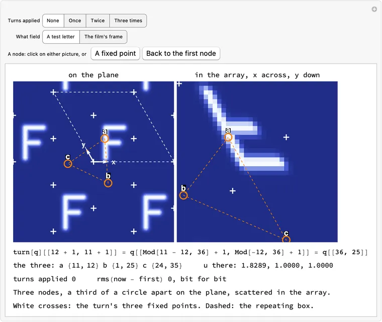
      

      Download ff-noise.wl

      White noise beside the frame it lands on, above the measured share of seeds that reach the film against the noise size, flat at one from 3e-9 to 4.
      What this draws, in Wolfram 15.0, 00:02
      def find_film(q, T=6.355, tol=1e-10):

      What: the first guess of the period. It is the 's own clock: , the time a small disturbance takes to swing once round it.

      Why: at the start the field is small, and every small wave in it swings at this one period, whatever its shape, because both chemicals diffuse alike. It is also close: the film's period is 6.3902, and a uniform swing at full size takes 6.4276.

      Try it: move and watch the clock, move the start and see where ends

      Orange: a tick every . Blue rings: a tick every start below.

      growth rate

      Measured at , 20 seeds a row.

      ends: sweeps

      Where comes from, and why every wave shares it

      For one uniform cell, , . At the rest state the Jacobian is

      Its eigenvalues are , with and . At , : , , , which the code rounds to . Above the rest state is unstable, which is why anything grows at all. is smallest at , where it is , and rises either way (find-film-modes.json, block m9_rest).

      Now a wave on the mesh, with its wave vector, a complex amplitude and an eigenvector of . The reaction linearised is and diffusion is the mesh Laplacian times the diffusion constant, which is the same number for both chemicals (rate applies one Laplacian to , both components). So the wave sees : the same eigenvectors, the same , and growth . Pattern and clock separate. Had the chemicals diffused at different rates, each wave would have its own clock, and no one guess could fit them all. The true r33₁3₂ film of section 15 has , and the program does fail there, but for another reason: its free period lets its unison mode win (the card on the raise).

      Measured on the real program: one sweep at from rest plus a single wave, against the formula, over 19 waves: worst relative error .

      Why the value matters a little, and how little: the table

      What it is really for. At this a third of a swing is : waves that tick at land at the angle of the zeros of the average (the card on the filter). So from the very first sweep the average does its job. The readout above shows that angle for any start.

      It need not be right. Any start from to reaches the film, 20 of 20 at each value, and from to it costs at most 28 sweeps against 26. At it is even a sweep quicker. The code's value is the natural one, not a needed one. It does not stay either: on seed 1, goes 6.355, 6.455, 6.355, 6.335, 6.435, 6.429, 6.392 over its first sweeps (the card on the clip).

      Start Ends (of 20)Median sweeps
      to near , 20: a flat field, returned with no error13.5, 21
      the film, 11; near , 944
      the film, 2040.5
      the film, 2026
      the film, 2042.5
      the film, 13; , 746
      , 2018
      three uniform cycles, , 20: flat, returned with no error10
      , 2022

      Seeds 14001-14020, find-film-runs.json, block R9.

      Why that staircase. The rule the program tests is slide, with meaning simulate over time . On the film that holds at , and also at , and for the film turned by at , since sliding twice is sliding once backwards ( on the exact frame). At it holds for neither: a third of it is a whole period, and slid, that does not match. There the uniform cycle wins, since on a flat field a slide does nothing and any whole number of cycles in passes. And near the rule passes trivially on a flat field, since of time changes nothing. So the program does not ask for the shortest period. It asks for a the rule accepts, and a start far off can find a different one.

      Mathematica
      (* T = 6.355 is the rest state's own clock, 2 Pi/omega. Left: one cell's two chemicals spiralling out from rest, with a tick every 2 Pi/omega falling on one ray; slider b moves the clock. Right: where T ends against where it starts, measured; that slider picks a row. Run really runs the program from that T. Instant on an M5; Run takes 2 s or so at T near 6, more at large T. Noise comes from Wolfram's generator. *)
      n = 36; box = 40.;   (* a triangular mesh of n x n nodes, in a repeating box of this side *)
      a = 1.; b = 2.3;     (* the Brusselator's constants; both chemicals diffuse at rate 1 *)
      dt = 0.02;           (* the longest time step *)
      
      (* How fast the chemicals q = {u, v} are changing: diffusion plus reaction. *)
      laplacian[f_] := 2/(3 (box/n)^2) ListCorrelate[{{1, 1, 0}, {1, -6, 1}, {0, 1, 1}}, f, {2, 2}];
      rate[{u_, v_}] := {laplacian[u] + a - (b + 1) u + u^2 v, laplacian[v] + b u - u^2 v};
      
      (* Run time forward by t (fourth-order Runge-Kutta). *)
      simulate[q0_, t_] := Module[{q = q0, steps = Ceiling[t/dt], h, k1, k2, k3, k4},
         h = t/steps;
         Do[
          k1 = rate[q];
          k2 = rate[q + h/2 k1];
          k3 = rate[q + h/2 k2];
          k4 = rate[q + h k3];
          q += h/6 (k1 + 2 k2 + 2 k3 + k4),
          {steps}];
         q];
      
      (* Slide the picture by a third of the box. On the film this costs T/3 of time. *)
      slide[q_] := RotateLeft[q, {0, n/3, 2 n/3}];
      
      (* Turn the picture 120 degrees about the origin. On the film this costs no time. *)
      turn[q_] := Table[f[[Mod[x - y, n] + 1, Mod[-y, n] + 1]], {f, q}, {y, 0, n - 1}, {x, 0, n - 1}];
      
      (* One frame of the film, its period T, and the number of sweeps it took. *)
      findFilm[q0_, T0_ : 6.355, tol_ : 1*^-10] := Module[{q, T = T0, third, twoThirds, lag, speed},
         q = (q0 + turn[q0] + turn[turn[q0]])/3;    (* costs no time, so impose it once and it stays *)
         Do[
          q = simulate[q, T];                       (* one free period: what decays, decays *)
          third = simulate[q, T/3];
          twoThirds = simulate[third, T/3];
      
          lag = slide[third] - q;                   (* zero on the film *)
          If[RootMeanSquare[Flatten[lag]] < tol, Return[{q, T, sweep}, Module]];
      
          (* T is off by 3 x lag / speed. Move it gently, since at first it's all noise. *)
          speed = rate[q];
          T -= Clip[3 Total[lag speed, 3]/Total[speed speed, 3], {-0.1, 0.1}];
      
          (* What obeys the rule survives the average; what ticks in unison cancels. *)
          q = (q + slide[third] + slide[slide[twoThirds]])/3,
          {sweep, 399}];
         $Failed];
      
      (* Start from the rest state plus white noise, and find the film. *)
      rest = {ConstantArray[a, {n, n}], ConstantArray[b/a, {n, n}]};
      noise[s_, amp_ : 0.1] := (SeedRandom[s]; rest + RandomVariate[NormalDistribution[0, amp], {2, n, n}]);
      
      (* The rest state's clock: the Jacobian there has trace b - 1 - a^2 and determinant a^2, so its eigenvalues are sigma + i omega. *)
      gsSigma[bb_] := (bb - 1 - a^2)/2;
      gsOmega[bb_] := Sqrt[a^2 - gsSigma[bb]^2];
      gsClock[bb_] := 2 Pi/gsOmega[bb];
      
      (* One cell, no diffusion: the path from a small disturbance, and where it is at time t. *)
      gsCell[bb_, start_, tEnd_] := Module[{u, v, t}, NDSolveValue[{u'[t] == a - (bb + 1) u[t] + u[t]^2 v[t], v'[t] == bb u[t] - u[t]^2 v[t], u[0] == a + start, v[0] == bb/a},
          {u, v}, {t, 0, tEnd}, PrecisionGoal -> 10, AccuracyGoal -> 10]];
      
      (* The phase plane. Close up, the path stops where it first leaves the view: later it comes back at full size, where the linear picture no longer holds. Orange: a tick every 2 Pi/omega. Blue rings: a tick every start T. *)
      gsPlane[bb_, T0_, close_] := Module[{clock = gsClock[bb], f, box2, path, tStop, ticks, start},
         start = If[close, If[bb > 2.02, 0.005, 0.05], If[bb > 2.02, 0.06, 0.75]];
         f = gsCell[bb, start, 8 clock];
         path = Table[{f[[1]][t], f[[2]][t]}, {t, 0., 8 clock, 0.01}];
         box2 = If[close, {{a - 0.12, a + 0.12}, {bb/a - 0.2, bb/a + 0.2}}, MinMax /@ Transpose[path]];
         tStop = If[close, 0.01 (LengthWhile[path, box2[[1, 1]] <= #[[1]] <= box2[[1, 2]] && box2[[2, 1]] <= #[[2]] <= box2[[2, 2]] &] - 1), 8 clock];
         ticks[dt_] := Table[{f[[1]][t], f[[2]][t]}, {t, 0., tStop, dt}];
         Graphics[{
           {GrayLevel[0.6], Line[Take[path, UpTo[Round[tStop/0.01] + 1]]]},
           {Dashed, Gray, Line[{{a, bb/a}, {a + 40 start, bb/a}}]},
           If[Abs[T0 - clock] > 0.002, {RGBColor[0.2, 0.3, 0.8], AbsolutePointSize[10], Point[ticks[T0]], White, AbsolutePointSize[6], Point[ticks[T0]]}, {}],
           {Orange, AbsolutePointSize[7], Point[ticks[clock]]},
           {Black, Thick, Text[Style["+", 18], {a, bb/a}]}},
          Frame -> True, FrameLabel -> {"u", "v, one cell, no diffusion"}, PlotRange -> box2, PlotRangePadding -> Scaled[0.04], AspectRatio -> 1, ImageSize -> 340]];
      
      (* Three waves near rest: each sees J - k^2, so the same clock and its own growth. lam is the mesh Laplacian's eigenvalue on the wave. *)
      gsWaves = {{"flat", 0, 0, Automatic}, {"long", 1, 0, Automatic}, {"short", 2, 1, Dashed}};
      gsLam[m_, l_] := 2/(3 (box/n)^2) (2 Cos[2 Pi m/n] + 2 Cos[2 Pi l/n] + 2 Cos[2 Pi (m + l)/n] - 6);
      gsWave[bb_, lam_, t_] := With[{s = gsSigma[bb], w = gsOmega[bb]}, 0.03 Exp[(s + lam) t] {Cos[w t] + Sin[w t] (bb - 1 - s)/w, -bb Sin[w t]/w}];
      gsFactor[bb_, lam_] := Exp[(gsSigma[bb] + lam) gsClock[bb]];
      gsThree[bb_] := Module[{clock = gsClock[bb], rest0 = {a, bb/a}, view = {{-0.12, 0.12}, {-0.2, 0.2}}, inside},
         inside[p_] := Abs[p[[1]]] < 0.12 && Abs[p[[2]]] < 0.2;
         Graphics[{
           {Dashed, Gray, Line[{rest0, rest0 + {0.12, 0}}]},
           Table[With[{lam = gsLam[w[[2]], w[[3]]]}, {
              {If[w[[1]] === "flat", RGBColor[0.2, 0.3, 0.8], GrayLevel[0.5]], If[w[[4]] === Dashed, Dashed, Thick], Line[rest0 + # & /@ TakeWhile[Table[gsWave[bb, lam, t], {t, 0., 4 clock, 0.02}], inside]]},
              {Orange, AbsolutePointSize[7], Point[rest0 + # & /@ Select[Table[gsWave[bb, lam, k clock], {k, 0, 4}], inside]]}}], {w, gsWaves}],
           {Black, Thick, Text[Style["+", 18], rest0]}},
          Frame -> True, FrameLabel -> {"u at a peak of the wave", "v there"}, PlotRange -> rest0 + view, AspectRatio -> 1, ImageSize -> 340]];
      
      (* Measured with the Python over seeds 14001-14020, not recomputed here: {start T, median end T, median sweeps, {on the film, at twice its period, at four times, flat at three uniform cycles, T near 0}}. *)
      gsTable = {{1, 0., 13.5, {0, 0, 0, 0, 20}}, {2, 0., 21, {0, 0, 0, 0, 20}}, {3, 0., 33.5, {1, 0, 0, 0, 19}}, {3.5, 6.39016, 44, {11, 0, 0, 0, 9}}, {4, 6.39016, 40.5, {20, 0, 0, 0, 0}},
         {4.5, 6.39016, 34, {20, 0, 0, 0, 0}}, {5, 6.39016, 31, {20, 0, 0, 0, 0}}, {5.5, 6.39016, 28, {20, 0, 0, 0, 0}}, {6, 6.39016, 26, {20, 0, 0, 0, 0}}, {6.355, 6.39016, 26, {20, 0, 0, 0, 0}},
         {7, 6.39016, 25, {20, 0, 0, 0, 0}}, {7.5, 6.39016, 28, {20, 0, 0, 0, 0}}, {8, 6.39016, 32, {20, 0, 0, 0, 0}}, {8.5, 6.39016, 38, {20, 0, 0, 0, 0}}, {9, 6.39016, 42.5, {20, 0, 0, 0, 0}},
         {9.25, 6.39016, 44, {17, 3, 0, 0, 0}}, {9.5, 6.39016, 46, {13, 7, 0, 0, 0}}, {9.75, 12.78032, 40, {6, 14, 0, 0, 0}}, {10, 12.78032, 38, {0, 20, 0, 0, 0}}, {11, 12.78032, 26, {0, 20, 0, 0, 0}},
         {12, 12.78032, 18, {0, 20, 0, 0, 0}}, {13, 12.78032, 16, {0, 20, 0, 0, 0}}, {14, 12.78032, 26, {0, 14, 0, 5, 0, 1}}, {15, 19.28286, 49.5, {0, 2, 0, 18, 0}}, {16, 19.28286, 39, {0, 0, 0, 20, 0}},
         {17, 19.28286, 26, {0, 0, 0, 20, 0}}, {18, 19.28286, 18, {0, 0, 0, 20, 0}}, {19, 19.28286, 10, {0, 0, 0, 20, 0}}, {19.17, 19.28286, 10, {0, 0, 0, 20, 0}}, {20, 19.28286, 11, {0, 0, 0, 20, 0}},
         {21, 19.28286, 21, {0, 0, 0, 20, 0}}, {22, 19.28286, 31, {0, 0, 0, 20, 0}}, {24, 19.28286, 53, {0, 0, 1, 19, 0}}, {26, 25.56064, 22, {0, 0, 20, 0, 0}}};
      gsEnds[row_] := With[{c = PadRight[row[[4]], 6]}, Row[{StringRiffle[Pick[MapThread[ToString[#1] <> " " <> #2 &, {c, {"on the film", "at twice its period", "at four times its period", "flat, at three uniform cycles", "with T near 0", "raised"}}], # > 0 & /@ c], ", "], ", of 20"}]];
      gsStairs[row_] := ListLinePlot[gsTable[[All, {1, 2}]], Mesh -> All, PlotRange -> {{0, 27}, {-1, 27}}, AxesLabel -> {"where T starts", "where T ends"}, ImageSize -> 340, AspectRatio -> 1,
         GridLines -> {{row[[1]]}, {6.39016, 12.78032, 19.28286, 25.56064}}, GridLinesStyle -> Directive[Gray, Dashed],
         Epilog -> {Orange, PointSize[0.02], Point[row[[{1, 2}]]], Black, Text["the film", {1, 6.39016}, {-1, -1}], Text["2 x", {1, 12.78032}, {-1, -1}], Text["3 uniform cycles", {1, 19.28286}, {-1, -1}], Text["4 x", {1, 25.56064}, {-1, -1}]}];
      
      (* Run the real program from this T, at the program's own b. T can pass through 0 at low starts, where simulate divides by zero steps and hands q back, hence the Quiet. *)
      gsRun[T0_] := Module[{r = Quiet[findFilm[noise[1], N[T0]], {Power::infy, Infinity::indet}]},
         Row[{"Live, seed 1 at b = 2.3, from T = ", T0, ": T ends ", If[Abs[r[[2]]] < 1*^-6, "near 0", Row[{"at ", NumberForm[r[[2]], 8]}]], " after ", r[[3]], " sweeps."}]];
      
      gsView[bb_, rowIndex_, view_, live_] := With[{row = gsTable[[rowIndex]], clock = gsClock[bb]}, Column[{
           Row[{If[view === "waves", gsThree[bb], gsPlane[bb, row[[1]], view === "close"]], gsStairs[row]}, "  "],
           Row[{"2 Pi/omega = ", NumberForm[clock, {4, 3}], "     growth rate sigma = ", NumberForm[gsSigma[bb], {3, 2}], "     omega T/3 = ", NumberForm[gsOmega[bb] row[[1]]/3 180/Pi, {4, 1}], " degrees"}],
           Row[{"Start T = ", row[[1]], " ends: ", gsEnds[row], "     median sweeps ", row[[3]]}],
           "Orange: a tick every 2 Pi/omega. Blue rings: a tick every start T. The staircase is measured at b = 2.3, 20 seeds a row.",
           Which[live =!= None, live,
            view === "waves", Row[{"A flat wave, a long wave and a short one, each with its own growth a tick: x", NumberForm[gsFactor[bb, 0.], {6, 2}], ", x", NumberForm[gsFactor[bb, gsLam[1, 0]], {6, 2}], ", x", NumberForm[gsFactor[bb, gsLam[2, 1]], {6, 2}], ". All their ticks fall on the one dashed ray: one clock, whatever the shape."}],
            bb < 2, "Below b = 2 the rest state is stable, and the disturbance spirals in. The clock still ticks.",
            bb <= 2.02, "At b = 2 the swing neither grows nor shrinks, at first.",
            view === "close", Row[{"Close up: while the disturbance is small, every orange tick falls on the dashed ray: exactly one turn per tick, and x", NumberForm[gsFactor[bb, 0.], {6, 2}], " larger each time."}],
            True, "At full size the ticks fall behind: a large swing takes longer, 6.428 at b = 2.3."]}, Spacings -> 1]];
      
      Manipulate[
       gsView[bb, First[FirstPosition[gsTable[[All, 1]], T0]], view, If[live[[1]] === T0 && bb == 2.3, live[[2]], None]],
       {{live, {0, None}}, ControlType -> None},
       {{bb, 2.3, "b, the constant in the reaction"}, 1.5, 3.5, 0.05, Appearance -> "Labeled"},
       {{T0, 6.355, "Where T starts"}, gsTable[[All, 1]], ControlType -> Manipulator, Appearance -> "Labeled"},
       {{view, "close", "How close to look"}, {"close" -> "Close up", "whole" -> "The whole swing", "waves" -> "Three shapes of wave"}, SetterBar},
       Row[{Button["Run from this T", live = {T0, Row[{"Running from T = ", T0, "..."}]}; live = {T0, gsRun[T0]}, Method -> "Queued"]}],
       SaveDefinitions -> True]
      

      Download ff-guess.wl

      One cell spiralling out from rest with orange ticks on a dashed ray, beside the measured staircase of where T ends against where it starts.
      What this draws, in Wolfram 15.0, 00:01

      19. The symmetry that costs no time

      return q[:, (x - y) % N, -y % N]

      What: turn fills each node from another node, picked by whole-number arithmetic: the new is the old , wrapped round the box.

      Why: a turn carries this mesh exactly onto itself, so the turn needs no interpolation. Nothing is smeared, no number changes, and three turns give back the same bits.

      Try it: tap a node, then apply the turn

      on the plane

      in the array

      White crosses: the turn's three fixed points. Dashed: the repeating box.

      the three, as : there:

      turns applied rms(now first)

      The formula, derived; and how to read the Python

      A node sits on the plane at , with along the row and at from it, each of length . A clockwise turn by takes and : both whole-number combinations. So what sits at moves to :

      turn needs the reverse: which old node fills the new ? Solving gives . That is the line. The array is indexed row first, so

      y, x = np.indices((N, N))

      makes two arrays, rows first, and q[:, (x - y) % N, -y % N] asks, for each new node, for row and column , for both chemicals (the :). -y % N reads as , and Python's % never returns a negative number, which is what makes the wrap-around come out. Checked against the page's map at every node: difference 0 (find-film-modes.json, block m2_commute).

      The box wraps as a whole: is itself a wrap of the box, so the turn is well defined on the repeating box.

      Why no interpolation matters, and the three fixed points

      Only this mesh allows it. On a square mesh a turn by lands between nodes. A value there has to be interpolated, which smooths the field and is not exactly undone by two more turns: the average of the three copies would then not be exactly symmetric, and rate would not commute with it. Here the turn is a permutation of the array: three applications are the identity bit for bit (difference 0), and the commutators on the card on why it stays reach round-off.

      The fixed points. A node comes back to itself when and , that is : on this mesh these are , and , found by brute force. They are the slide's vector and its double: the turn fixes up to a wrap of the box, which is why slide and turn commute. On the repeating box the turn about the origin is therefore also a turn about each of the other two, so the origin is not special. All three are of section 9's kind , where the turn costs no time; its kinds and are other nodes, such as and . If were not divisible by only the origin would be fixed, and the slide could not be written either.

      The test letter is a picture for this card only. The program's turn never sees it.

      Mathematica
      (* turn[q] fills each node from another, by whole-number arithmetic. Click a node to see its three images, on the plane and in the array; apply the turn: the picture really turns on the plane and shears in the array, and three turns give back the same bits. About 4 s on an M5, for the letter and the film's frame. *)
      n = 36; box = 40.;   (* a triangular mesh of n x n nodes, in a repeating box of this side *)
      a = 1.; b = 2.3;     (* the Brusselator's constants; both chemicals diffuse at rate 1 *)
      dt = 0.02;           (* the longest time step *)
      
      (* How fast the chemicals q = {u, v} are changing: diffusion plus reaction. *)
      laplacian[f_] := 2/(3 (box/n)^2) ListCorrelate[{{1, 1, 0}, {1, -6, 1}, {0, 1, 1}}, f, {2, 2}];
      rate[{u_, v_}] := {laplacian[u] + a - (b + 1) u + u^2 v, laplacian[v] + b u - u^2 v};
      
      (* Run time forward by t (fourth-order Runge-Kutta). *)
      simulate[q0_, t_] := Module[{q = q0, steps = Ceiling[t/dt], h, k1, k2, k3, k4},
         h = t/steps;
         Do[
          k1 = rate[q];
          k2 = rate[q + h/2 k1];
          k3 = rate[q + h/2 k2];
          k4 = rate[q + h k3];
          q += h/6 (k1 + 2 k2 + 2 k3 + k4),
          {steps}];
         q];
      
      (* Slide the picture by a third of the box. On the film this costs T/3 of time. *)
      slide[q_] := RotateLeft[q, {0, n/3, 2 n/3}];
      
      (* Turn the picture 120 degrees about the origin. On the film this costs no time. *)
      turn[q_] := Table[f[[Mod[x - y, n] + 1, Mod[-y, n] + 1]], {f, q}, {y, 0, n - 1}, {x, 0, n - 1}];
      
      (* One frame of the film, its period T, and the number of sweeps it took. *)
      findFilm[q0_, T0_ : 6.355, tol_ : 1*^-10] := Module[{q, T = T0, third, twoThirds, lag, speed},
         q = (q0 + turn[q0] + turn[turn[q0]])/3;    (* costs no time, so impose it once and it stays *)
         Do[
          q = simulate[q, T];                       (* one free period: what decays, decays *)
          third = simulate[q, T/3];
          twoThirds = simulate[third, T/3];
      
          lag = slide[third] - q;                   (* zero on the film *)
          If[RootMeanSquare[Flatten[lag]] < tol, Return[{q, T, sweep}, Module]];
      
          (* T is off by 3 x lag / speed. Move it gently, since at first it's all noise. *)
          speed = rate[q];
          T -= Clip[3 Total[lag speed, 3]/Total[speed speed, 3], {-0.1, 0.1}];
      
          (* What obeys the rule survives the average; what ticks in unison cancels. *)
          q = (q + slide[third] + slide[slide[twoThirds]])/3,
          {sweep, 399}];
         $Failed];
      
      (* Start from the rest state plus white noise, and find the film. *)
      rest = {ConstantArray[a, {n, n}], ConstantArray[b/a, {n, n}]};
      noise[s_, amp_ : 0.1] := (SeedRandom[s]; rest + RandomVariate[NormalDistribution[0, amp], {2, n, n}]);
      
      (* Four points a mesh step, linear on the mesh's own triangles, as the page paints: a turned field then draws as the turned picture. *)
      meshTent = Table[Max[0., 1. - Max[Abs[i], Abs[j], Abs[i - j]]/4.], {j, -3, 3}, {i, -3, 3}];
      meshFine[f_] := ListCorrelate[meshTent, KroneckerProduct[f, Normal[SparseArray[{{1, 1} -> 1.}, {4, 4}]]], {4, 4}];
      
      (* A field on the plane, as a picture: the mesh's two axes are 120 degrees apart. Blue is lo, white is hi. *)
      picture[u_, {lo_, hi_}, size_ : 240] := Colorize[
         Quiet[    (* Wolfram 15's ImageTransformation trips on the notebook's light/dark background, harmlessly *)
          ImageTransformation[Image[Rescale[Reverse[meshFine[u]], {lo, hi}]],
           {#[[1]] + #[[2]]/Sqrt[3.], 2 #[[2]]/Sqrt[3.]}/box + 0.5/(4 n) &, {size, size},
           DataRange -> {{0, 1}, {0, 1}}, PlotRange -> {{-40., 40.}, {-40., 40.}},
           Padding -> "Periodic", Resampling -> "Linear"],
          RemoveAlphaChannel::imginv],
         ColorFunction -> (Blend[{RGBColor[0.118, 0.165, 0.51], RGBColor[0.251, 0.329, 0.808], RGBColor[0.588, 0.667, 0.941], RGBColor[0.961, 0.973, 1.]}, #] &), ColorFunctionScaling -> False];
      
      (* A test field, not what the program gets: the letter F drawn upright on the plane, in u. *)
      tmWorld[{i_, j_}] := {box (i - j/2)/n, box Sqrt[3.]/2 j/n};
      tmLetter = Module[{d = RegionDistance[RegionUnion[Line[{{6, 2}, {6, 17}, {15, 17}}], Line[{{6, 9.5}, {12.5, 9.5}}]]]},
         {rest[[1]] + Table[0.9 Exp[-Min[Table[d[tmWorld[{x + da, y + db}]], {da, {-n, 0, n}}, {db, {-n, 0, n}}]]^2/2.4], {y, 0, n - 1}, {x, 0, n - 1}], rest[[2]]}];
      tmFilm = First[findFilm[noise[1]]];
      tmFields[input_] := NestList[turn, If[input === "letter", tmLetter, tmFilm], 3];
      
      (* Where turn sends what sits at (i, j), by (turn[q])[[y + 1, x + 1]] = q[[Mod[x - y, n] + 1, Mod[-y, n] + 1]]. *)
      tmImage[{i_, j_}] := {Mod[j - i, n], Mod[-i, n]};
      tmFixed = {{0, 0}, {24, 12}, {12, 24}};
      tmValue[u_, {x_, y_}] := u[[y + 1, x + 1]];
      (* The periodic copy of a node nearest the origin, so the turn about the origin stays in view; then a place in a picture's pixels. *)
      tmNearest[{x_, y_}] := First[MinimalBy[Flatten[Table[{x + da, y + db}, {da, {-n, 0, n}}, {db, {-n, 0, n}}], 1], Norm[tmWorld[#]] &]];
      tmOnPlane[node_] := 480 (tmWorld[node] + 40)/80;
      tmInArray[{x_, y_}] := 480 {x + 0.5, n - y - 0.5}/n;
      (* Inverses of those two, for a click. *)
      tmFromPlane[{px_, py_}] := With[{wx = 80 px/480 - 40, wy = 80 py/480 - 40}, With[{lj = wy/(box Sqrt[3.]/2)}, Mod[Round[{wx/box + lj/2, lj} n], n]]];
      tmFromArray[{px_, py_}] := Mod[Floor[{px, 480 - py} n/480], n];
      tmArrayImage[u_, {lo_, hi_}] := Colorize[ImageResize[Image[Rescale[u, {lo, hi}]], {480, 480}, Resampling -> "Nearest"], ColorFunction -> (Blend[{RGBColor[0.118, 0.165, 0.51], RGBColor[0.251, 0.329, 0.808], RGBColor[0.588, 0.667, 0.941], RGBColor[0.961, 0.973, 1.]}, #] &), ColorFunctionScaling -> False];
      
      (* The repeating box dashed, and which way x and y run on the plane. *)
      tmPlaneMarks = {{White, Dashed, Line[tmOnPlane /@ {{0, 0}, {n, 0}, {n, n}, {0, n}, {0, 0}}]},
         {White, Thick, Arrow[{tmOnPlane[{0, 0}], tmOnPlane[{7, 0}]}], Arrow[{tmOnPlane[{0, 0}], tmOnPlane[{0, 7}]}], Text[Style["x", 13, White], tmOnPlane[{9, 0}]], Text[Style["y", 13, White], tmOnPlane[{0, 9}]]}};
      
      (* The three rings a, b, c, dashed between; white crosses at the turn's fixed points. *)
      tmMarks[points_, fixedPoints_, fixed_] := {
         {White, Thick, Line[{# - {7, 0}, # + {7, 0}}], Line[{# - {0, 7}, # + {0, 7}}]} & /@ fixedPoints,
         {Orange, Dashed, Line[Append[points, First[points]]]},
         {Orange, Thick, Circle[#, 11] & /@ points},
         If[fixed, {}, MapThread[Text[Style[#1, 15, Bold, White, Background -> Black], #2 + {0, 22}] &, {{"a", "b", "c"}, points}]]};
      
      tmView[input_, node_, turns_, set_] := Module[{fields = tmFields[input], u, range, nodes, fixed, spots, x = node[[1]], y = node[[2]], dist},
         u = fields[[turns + 1, 1]];
         range = If[input === "letter", {0.98, 1.8}, MinMax[u]];
         nodes = NestList[tmImage, node, 2];
         fixed = nodes[[1]] === nodes[[2]];
         spots = NestList[{#[[2]] - #[[1]], -#[[1]]} &, tmNearest[node], 2];
         dist = RootMeanSquare[Flatten[fields[[turns + 1]] - fields[[1]]]];
         Column[{
           Grid[{{"on the plane", "in the array, x across, y down"}, {
              ClickPane[Show[picture[u, range, 480], Graphics[tmPlaneMarks], Graphics[tmMarks[tmOnPlane /@ spots, Flatten[Table[tmOnPlane[f + {da, db}], {f, tmFixed}, {da, {-n, 0, n}}, {db, {-n, 0, n}}], 2], fixed]], PlotRange -> {{0, 480}, {0, 480}}, ImageSize -> 300], (set[tmFromPlane[#]] &)],
              ClickPane[Show[tmArrayImage[u, range], Graphics[tmMarks[tmInArray /@ nodes, tmInArray /@ tmFixed, fixed]], PlotRange -> {{0, 480}, {0, 480}}, ImageSize -> 300], (set[tmFromArray[#]] &)]}}],
           Style[Row[{"turn[q][[", y, " + 1, ", x, " + 1]] = q[[Mod[", x, " - ", y, ", 36] + 1, Mod[-", y, ", 36] + 1]] = q[[", Mod[x - y, n] + 1, ", ", Mod[-y, n] + 1, "]]"}], FontFamily -> "Courier"],
           Row[{"the three: ", If[fixed, Row[{"one node ", node}], Row[MapThread[Row[{#1, " ", #2}] &, {{"a", "b", "c"}, nodes}], "  "]], "     u there: ", If[fixed, NumberForm[tmValue[u, node], {5, 4}], Row[Riffle[NumberForm[tmValue[u, #], {5, 4}] & /@ nodes, ", "]]]}],
           Row[{"turns applied ", turns, "     rms(now - first) ", If[dist === 0., "0, bit for bit", ScientificForm[dist, 2]]}],
           Which[fixed, "A fixed point of the turn: its three images are one node. On the plane they are three periodic copies of it.",
            input === "film", "The film's frame: the three nodes hold the same value, and turning changes nothing but round-off.",
            turns == 0, "Three nodes, a third of a circle apart on the plane, scattered in the array.",
            turns < 3, "What was at a is now at b, and so on round. On the plane the letter has turned, undistorted; in the array the same numbers have been sheared.",
            True, "Three turns: the same bits as at the start."],
           "White crosses: the turn's three fixed points. Dashed: the repeating box."}, Spacings -> 1]];
      
      Manipulate[
       tmView[input, node, turns, (node = #) &],
       {{node, {11, 12}}, ControlType -> None},
       {{turns, 0, "Turns applied"}, {0 -> "None", 1 -> "Once", 2 -> "Twice", 3 -> "Three times"}, SetterBar},
       {{input, "letter", "What field"}, {"letter" -> "A test letter", "film" -> "The film's frame"}, SetterBar},
       Row[{"A node: click on either picture, or  ", Button["A fixed point", node = {24, 12}], Button["Back to the first node", node = {11, 12}]}, " "],
       SaveDefinitions -> True]
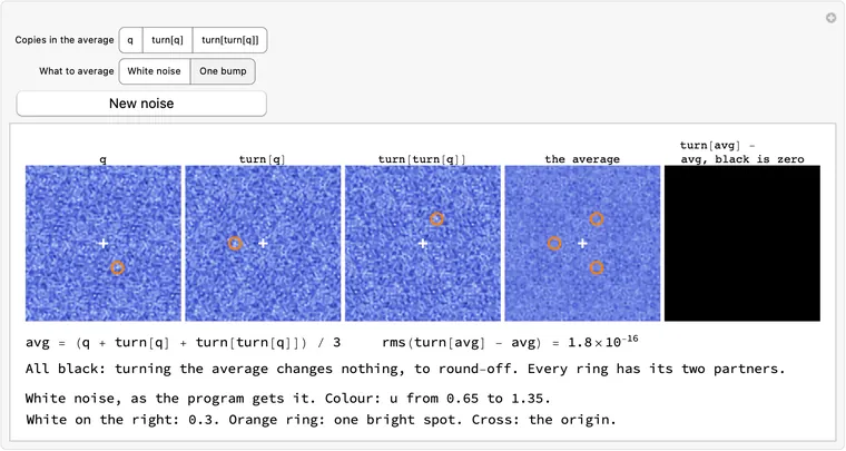
      

      Download ff-turn-map.wl

      A test letter on the plane and the same numbers sheared in the array, with three ringed nodes a third of a circle apart on the plane and scattered in the array.
      What this draws, in Wolfram 15.0, 00:04
      q = (q + turn(q) + turn(turn(q))) / 3

      What: the field is replaced by the average of itself and its two copies turned by about the origin. The result looks the same turned: every feature has two partners.

      Why: every frame of the film looks the same turned, so this symmetry costs no time: it can be demanded at once, with no simulation. Without this line the same program mostly finds a different film.

      Try it: switch the copies on and off

      q

      turn(q)

      turn(turn(q))

      the average

      turn(avg) - avg, black is zero

      Orange ring: one bright spot. Cross: the origin.

      rms(turn(avg) - avg)

      Why three copies, and only three, give zero

      Write for turn. Three turns are the identity: , exactly, since only moves numbers between places (0 difference, bit for bit; find-film-modes.json, block m2_commute). So for , the average of the three copies, : turning the average gives the average.

      With two copies, turns into , which differs from it by . And is turned, the same size. So on noise one copy leaves 0.1397, two exactly half of that, 0.0699, and three (seed 1; seeds 1-20 reach at most ; find-film-extra-lab.json).

      The last number is not zero only because and can round differently; the turn itself moves bits and loses none.

      The picture is on the plane; the array's own view of the turn, and why it needs no interpolation, is the card on turn(q). The turn's centre is the origin of the mesh; the cross marks it in the panes.

      It is a projection: what is thrown away, and how much

      , since gives . Applying the line twice changes nothing but round-off ( at most over seeds 1-20). So is a projection, onto the fields the turn leaves alone, and it is the nearest such field: is symmetric because is 's transpose.

      How big that space is: the turn fixes 3 of the 1296 nodes, the origin and two more, and groups the others in threes, so 434 values per chemical remain free: 868 numbers of 2592. White noise keeps that share of its power, 33.5%, so its size falls from to a predicted 0.0579: measured 0.0581, the median of seeds 1-20. That is why the average pane looks calmer on the same colour scale. The mean does not move, beyond .

      What the line does to the run, measured

      Removed, on seeds 5001-5400: 373 of 400 land on one plane wave, a different film with that obeys the slide rule just as well, in about 44 sweeps; 27 of 400 land on the film, shifted off the mesh by a fraction of a step, after a median of 363 sweeps against 26, and 4 of them raise at sweep 399, a few sweeps short: the median counts their finish with the cap lifted.

      So the line does two things, and neither is to hold the film up. It rules the plane wave out, since a plane wave has no turn. And it removes the fields where a mode with sweep factor 0.9557 lives, which is why those 27 runs take so long. The film is stable without it: a kicked film returns even with the line removed (find-film-runs.json, block R2long).

      Imposing it once is enough. Repeating it after each average gives the same run: 40 of 40 seeds, same sweeps (the card on why it stays).

      Mathematica
      (* The first line: q averaged with its two copies turned 120 degrees about the origin. Switch the copies on and off: turn[avg] - avg goes black, to round-off, only with all three. Instant on an M5. Noise comes from Wolfram's generator. *)
      n = 36; box = 40.;   (* a triangular mesh of n x n nodes, in a repeating box of this side *)
      a = 1.; b = 2.3;     (* the Brusselator's constants; both chemicals diffuse at rate 1 *)
      
      (* Turn the picture 120 degrees about the origin. On the film this costs no time. *)
      turn[q_] := Table[f[[Mod[x - y, n] + 1, Mod[-y, n] + 1]], {f, q}, {y, 0, n - 1}, {x, 0, n - 1}];
      
      (* Start from the rest state plus white noise, and find the film. *)
      rest = {ConstantArray[a, {n, n}], ConstantArray[b/a, {n, n}]};
      noise[s_, amp_ : 0.1] := (SeedRandom[s]; rest + RandomVariate[NormalDistribution[0, amp], {2, n, n}]);
      
      (* Four points a mesh step, linear on the mesh's own triangles, as the page paints: a turned field then draws as the turned picture. *)
      meshTent = Table[Max[0., 1. - Max[Abs[i], Abs[j], Abs[i - j]]/4.], {j, -3, 3}, {i, -3, 3}];
      meshFine[f_] := ListCorrelate[meshTent, KroneckerProduct[f, Normal[SparseArray[{{1, 1} -> 1.}, {4, 4}]]], {4, 4}];
      
      (* A field on the plane, as a picture: the mesh's two axes are 120 degrees apart. Blue is lo, white is hi. *)
      picture[u_, {lo_, hi_}, size_ : 240] := Colorize[
         Quiet[    (* Wolfram 15's ImageTransformation trips on the notebook's light/dark background, harmlessly *)
          ImageTransformation[Image[Rescale[Reverse[meshFine[u]], {lo, hi}]],
           {#[[1]] + #[[2]]/Sqrt[3.], 2 #[[2]]/Sqrt[3.]}/box + 0.5/(4 n) &, {size, size},
           DataRange -> {{0, 1}, {0, 1}}, PlotRange -> {{-40., 40.}, {-40., 40.}},
           Padding -> "Periodic", Resampling -> "Linear"],
          RemoveAlphaChannel::imginv],
         ColorFunction -> (Blend[{RGBColor[0.118, 0.165, 0.51], RGBColor[0.251, 0.329, 0.808], RGBColor[0.588, 0.667, 0.941], RGBColor[0.961, 0.973, 1.]}, #] &), ColorFunctionScaling -> False];
      
      (* A test field, not what the program is given: one bump off to one side of the origin. *)
      taBump = Module[{c = Table[0.9 Exp[-Min[Table[With[{i = x + da - 8, j = y + db - 3}, i^2 + j^2 - i j], {da, {-n, 0, n}}, {db, {-n, 0, n}}]]/12], {y, 0, n - 1}, {x, 0, n - 1}]}, {rest[[1]] + c, rest[[2]]}];
      
      (* |u| on the plane, black is zero, white is hi: the geometry of picture. *)
      taSize[f_, hi_] := Quiet[ImageTransformation[Image[Clip[Abs[Reverse[meshFine[f]]]/hi, {0, 1}]], {#[[1]] + #[[2]]/Sqrt[3.], 2 #[[2]]/Sqrt[3.]}/box + 0.5/(4 n) &, {300, 300},
          DataRange -> {{0, 1}, {0, 1}}, PlotRange -> {{-40., 40.}, {-40., 40.}}, Padding -> "Periodic", Resampling -> "Linear"], RemoveAlphaChannel::imginv];
      
      (* What sits at node (i, j) in q appears at (j - i, -i) in turn[q]. A node's place in a picture's 300 pixels, for the rings and the cross. *)
      taTurned[{i_, j_}] := {j - i, -i};
      taPixel[{i_, j_}] := 300 ({box (i - j/2)/n, box Sqrt[3.]/2 j/n} + 40)/80;
      (* The brightest node at a distance from the origin where its turned copies stay in view. *)
      taSpot[u_] := First[MaximalBy[Select[Flatten[Table[{i, j}, {j, -17, 18}, {i, -17, 18}], 1], 6 <= Norm[{#[[1]] - #[[2]]/2, #[[2]] Sqrt[3.]/2}] <= 13 &], u[[Mod[#[[2]], n] + 1, Mod[#[[1]], n] + 1]] &]];
      taRings[spots_, r_] := {Orange, Thick, Circle[taPixel[#], r] & /@ spots, White, Thick, Line[taPixel[{0, 0}] + # & /@ {{-7, 0}, {7, 0}}], Line[taPixel[{0, 0}] + # & /@ {{0, -7}, {0, 7}}]};
      
      taView[on_, input_, seed_] := Module[{q, copies, names = {"q", "turn[q]", "turn[turn[q]]"}, use, avg, res, e, spot, spots, lo, hi, white, panel, r},
         q = If[input === "noise", noise[seed], taBump];
         copies = {q, turn[q], turn[turn[q]]};
         use = If[on === {}, {1}, Sort[on]];
         avg = Mean[copies[[use]]];
         res = turn[avg] - avg;
         e = RootMeanSquare[Flatten[res]];
         {lo, hi, white, r} = If[input === "noise", {0.65, 1.35, 0.3, 11}, {0.95, 1.6, 0.9, 18}];
         spot = If[input === "noise", taSpot[q[[1]]], {8, 3}];
         spots = NestList[taTurned, spot, 2];
         panel[title_, image_] := Labeled[Show[image, ImageSize -> 150], Style[title, 11, FontFamily -> "Courier"], Top];
         Column[{
           Grid[{Join[
              Table[panel[names[[k]], Show[picture[copies[[k, 1]], {lo, hi}, 300], Graphics[taRings[{spots[[k]]}, r]]]], {k, 3}],
              {panel["the average", Show[picture[avg[[1]], {lo, hi}, 300], Graphics[taRings[spots[[use]], r]]]],
               panel["turn[avg] - avg, black is zero", taSize[res[[1]], white]]}]}, Spacings -> 0.3],
           Row[{If[Length[use] == 1, Row[{"avg = ", names[[First[use]]]}], Row[{"avg = (", StringRiffle[names[[use]], " + "], ") / ", Length[use]}]], "     rms(turn[avg] - avg) = ", ScientificForm[e, 2]}],
           Switch[Length[use],
            3, "All black: turning the average changes nothing, to round-off. Every ring has its two partners.",
            2, "Not black: the average of two copies still changes when turned. The third partner is missing.",
            _, "One copy is just a turned picture: nothing has been averaged."],
           If[input === "noise", "White noise, as the program gets it. ", "One bump: a test field, not what the program gets. "] <> "Colour: u from " <> ToString[lo] <> " to " <> ToString[hi] <> ". White on the right: " <> ToString[white] <> ". Orange ring: one bright spot. Cross: the origin."}, Spacings -> 1]];
      
      Manipulate[
       taView[on, input, seed],
       {{seed, 1}, ControlType -> None},
       {{on, {1, 2, 3}, "Copies in the average"}, {1 -> "q", 2 -> "turn[q]", 3 -> "turn[turn[q]]"}, ControlType -> TogglerBar},
       {{input, "noise", "What to average"}, {"noise" -> "White noise", "bump" -> "One bump"}, SetterBar},
       Button["New noise", seed = seed + 1],
       SaveDefinitions -> True]
      

      Download ff-turn-avg.wl

      Noise and its two turned copies with a ring on one bright spot, their average with all three rings, and turn[avg] - avg all black.
      What this draws, in Wolfram 15.0, 00:01
      q = (q + turn(q) + turn(turn(q))) / 3           # costs no time, so impose it once and it stays

      What: the comment makes two claims. is why it can be done at the start. "It stays" is why the line never has to run again: from a symmetric field, every later field is symmetric too.

      Why: it stays because running a turned field gives the turned run. Nothing in the simulation prefers one of the mesh's three directions, so only round-off can break the symmetry, and at the program's noise it stays at round-off.

      Try it: run time forward, then change the start

      turn(q) - q, black is zero

      rms(turn(q) - q) on plain noise, run then turn against turn then run

      Seed 1. White in the right pane: .

      Why it stays: every piece of the program commutes with the turn

      Write for the turn. If each operation satisfies , then gives : maps symmetric fields to symmetric fields. So it is enough to check the pieces. (The chart is the Python's; the numbers under it are this page, live, and a check holds them together.)

      rate: the reaction acts node by node, so it does not care where a node is. The stencil's six neighbours are permuted by the turn in two three-cycles, and their negatives, so the sum over them is the same set of numbers in another order. simulate is built from rate and sums. slide commutes because its vector is fixed by the turn up to a wrap. The averages are sums of those.

      Commutator, rmsOn the exact frameOn plain noise
      turn with rate
      turn with simulate(q, T / 3)
      turn with simulate(q, T)
      turn with slide00

      The second column is the point: noise has no symmetry and the commutator is still round-off. It is a property of the operations, not of the field (find-film-modes.json, block m2_commute). The non-zero rows are only the order of the additions: the turn lists the neighbours in another order, and floating-point addition does not quite commute.

      The experiment that could have failed. Point the pair at the node itself, so that one direction of the mesh gets no diffusion. From the same symmetric start the residual leaves round-off at once, reaching 0.0081 after one period and 0.0163 after two, and the commutator is 0.0140 and 0.0267. With the six neighbours, over the same time, the residual is at most and the commutator on noise at most (find-film-extra-cardsA.json, block stays; script find_film_extra_cardsA.py). Nothing makes a field symmetric if it is not: without the line the noise's own residual falls from 0.1397 only because noise decays, and is still 0.0256 after one period and 0.0346 after two.

      "Costs no time", in numbers

      At one instant of the exact film, the turn's residual is : it holds with no simulation at all, so a single projection can impose it. The slide's, at that same instant, is 0.662, the size of the field's own change. It holds only a third of a period later (), and testing it takes 428 rate calls. Averaging over the slide alone, with no time step, would flatten the pattern: that is what the rest of the sweep has to pay for.

      How far "it stays" goes: where the comment needs a footnote

      Through a normal run, as far as round-off can tell. Seed 1: 0.1397 before the line, after it. The largest residual over all 25 sweeps, line by line: in q, in third, in speed, after the average. It is still after 120 sweeps past the stop. Imposing it every sweep changes nothing: 52 of 52 fresh seeds took the same sweeps, within , frames within .

      Not when the noise is tiny. Round-off stays small only if nothing amplifies it. A field of size has to grow about ten million times to reach the film's size, and the round-off that breaks the turn is carried up with it: the same three seeds take 55 sweeps (median) as written and 42 with the turn imposed every sweep. At noise , on the 53 of 100 seeds that reach the film, the residual ends between and (find-film-runs.json, block R10b). So "impose it once" is safe at the program's own , and it is a statement about that.

      Not for ever with no average. A returned frame, simulated on its own with no sweep at all: the residual grows from at period 50 to at period 150, about 1.015 a period, near the 1.015 of the modes that break the turn on the film. Round-off, but growing. The mode that takes the film to a uniform field gets there first, and it needs no broken symmetry (the card on what the frame cannot do).

      Mathematica
      (* "Impose it once and it stays": run time forward from three starts, watch turn[q] - q, and see that running then turning equals turning then running. A variant drops one direction of the mesh's stencil, and there the symmetry leaves round-off at once. About 1 s on an M5. Noise comes from Wolfram's generator. *)
      n = 36; box = 40.;   (* a triangular mesh of n x n nodes, in a repeating box of this side *)
      a = 1.; b = 2.3;     (* the Brusselator's constants; both chemicals diffuse at rate 1 *)
      dt = 0.02;           (* the longest time step *)
      
      (* How fast the chemicals q = {u, v} are changing: diffusion plus reaction. *)
      laplacian[f_] := 2/(3 (box/n)^2) ListCorrelate[{{1, 1, 0}, {1, -6, 1}, {0, 1, 1}}, f, {2, 2}];
      rate[{u_, v_}] := {laplacian[u] + a - (b + 1) u + u^2 v, laplacian[v] + b u - u^2 v};
      
      (* Run time forward by t (fourth-order Runge-Kutta). *)
      simulate[q0_, t_] := Module[{q = q0, steps = Ceiling[t/dt], h, k1, k2, k3, k4},
         h = t/steps;
         Do[
          k1 = rate[q];
          k2 = rate[q + h/2 k1];
          k3 = rate[q + h/2 k2];
          k4 = rate[q + h k3];
          q += h/6 (k1 + 2 k2 + 2 k3 + k4),
          {steps}];
         q];
      
      (* Slide the picture by a third of the box. On the film this costs T/3 of time. *)
      slide[q_] := RotateLeft[q, {0, n/3, 2 n/3}];
      
      (* Turn the picture 120 degrees about the origin. On the film this costs no time. *)
      turn[q_] := Table[f[[Mod[x - y, n] + 1, Mod[-y, n] + 1]], {f, q}, {y, 0, n - 1}, {x, 0, n - 1}];
      
      (* Start from the rest state plus white noise, and find the film. *)
      rest = {ConstantArray[a, {n, n}], ConstantArray[b/a, {n, n}]};
      noise[s_, amp_ : 0.1] := (SeedRandom[s]; rest + RandomVariate[NormalDistribution[0, amp], {2, n, n}]);
      
      (* Four points a mesh step, linear on the mesh's own triangles, as the page paints: a turned field then draws as the turned picture. *)
      meshTent = Table[Max[0., 1. - Max[Abs[i], Abs[j], Abs[i - j]]/4.], {j, -3, 3}, {i, -3, 3}];
      meshFine[f_] := ListCorrelate[meshTent, KroneckerProduct[f, Normal[SparseArray[{{1, 1} -> 1.}, {4, 4}]]], {4, 4}];
      
      (* A field on the plane, as a picture: the mesh's two axes are 120 degrees apart. Blue is lo, white is hi. *)
      picture[u_, {lo_, hi_}, size_ : 240] := Colorize[
         Quiet[    (* Wolfram 15's ImageTransformation trips on the notebook's light/dark background, harmlessly *)
          ImageTransformation[Image[Rescale[Reverse[meshFine[u]], {lo, hi}]],
           {#[[1]] + #[[2]]/Sqrt[3.], 2 #[[2]]/Sqrt[3.]}/box + 0.5/(4 n) &, {size, size},
           DataRange -> {{0, 1}, {0, 1}}, PlotRange -> {{-40., 40.}, {-40., 40.}},
           Padding -> "Periodic", Resampling -> "Linear"],
          RemoveAlphaChannel::imginv],
         ColorFunction -> (Blend[{RGBColor[0.118, 0.165, 0.51], RGBColor[0.251, 0.329, 0.808], RGBColor[0.588, 0.667, 0.941], RGBColor[0.961, 0.973, 1.]}, #] &), ColorFunctionScaling -> False];
      
      tsPeriod = 6.3901599;   (* the film's period, for the time axis only *)
      
      (* The program's stencil with the pair (1, 1), (-1, -1) pointed at the node itself: its four other neighbours, same constant. Not the program. *)
      tsLaplacian4[f_] := 2/(3 (box/n)^2) ListCorrelate[{{0, 1, 0}, {1, -4, 1}, {0, 1, 0}}, f, {2, 2}];
      tsRate4[{u_, v_}] := {tsLaplacian4[u] + a - (b + 1) u + u^2 v, tsLaplacian4[v] + b u - u^2 v};
      tsSimulate4[q0_, t_] := Module[{q = q0, steps = Ceiling[t/dt], h, k1, k2, k3, k4},
         h = t/steps;
         Do[
          k1 = tsRate4[q];
          k2 = tsRate4[q + h/2 k1];
          k3 = tsRate4[q + h/2 k2];
          k4 = tsRate4[q + h k3];
          q += h/6 (k1 + 2 k2 + 2 k3 + k4),
          {steps}];
         q];
      
      tsStart = noise[1];
      tsSym = (tsStart + turn[tsStart] + turn[turn[tsStart]])/3;
      (* 25 frames from 0 to 2 periods, from each start; and the same noise turned, to compare running then turning with turning then running. *)
      tsFrames[sim_, q0_] := NestList[sim[#, tsPeriod/12] &, q0, 24];
      tsRuns = <|"sym" -> tsFrames[simulate, tsSym], "unsym" -> tsFrames[simulate, tsStart], "four" -> tsFrames[tsSimulate4, tsSym]|>;
      tsTurned = <|"program" -> tsFrames[simulate, turn[tsStart]], "four" -> tsFrames[tsSimulate4, turn[tsStart]]|>;
      tsPlain = <|"program" -> tsRuns["unsym"], "four" -> tsFrames[tsSimulate4, tsStart]|>;
      tsResidual[q_] := RootMeanSquare[Flatten[turn[q] - q]];
      tsCurve = Map[tsResidual, tsRuns, {2}];
      tsCommutator[which_] := Table[RootMeanSquare[Flatten[tsTurned[which][[j]] - turn[tsPlain[which][[j]]]]], {j, 25}];
      
      (* |u| on the plane, black is zero, white is hi: the geometry of picture. *)
      tsSize[f_, hi_] := Quiet[ImageTransformation[Image[Clip[Abs[Reverse[meshFine[f]]]/hi, {0, 1}]], {#[[1]] + #[[2]]/Sqrt[3.], 2 #[[2]]/Sqrt[3.]}/box + 0.5/(4 n) &, {480, 480},
          DataRange -> {{0, 1}, {0, 1}}, PlotRange -> {{-40., 40.}, {-40., 40.}}, Padding -> "Periodic", Resampling -> "Linear"], RemoveAlphaChannel::imginv];
      
      tsView[which_, j_] := Module[{q = tsRuns[which][[j + 1]], comm = tsCommutator[If[which === "four", "four", "program"]][[j + 1]], times = Range[0, 24]/12.},
         Column[{
           Grid[{{Labeled[Image[picture[q[[1]], {0.65, 1.35}, 480], ImageSize -> 240], "q(t)", Top],
              Labeled[Image[tsSize[(turn[q] - q)[[1]], 0.03], ImageSize -> 240], "turn[q] - q, black is zero", Top]}}],
           ListLogPlot[Table[Transpose[{times, Clip[tsCurve[k], {1*^-17, Infinity}]}], {k, {"unsym", "four", "sym"}}], Joined -> True, PlotRange -> {{0, 2}, {1*^-17, 1}}, AxesLabel -> {"t, in periods", "rms(turn[q] - q)"},
            PlotStyle -> (If[#1 === which, Directive[RGBColor[0.2, 0.3, 0.8], Thick], GrayLevel[0.6]] & /@ {"unsym", "four", "sym"}), GridLines -> {{j/12.}, None}, GridLinesStyle -> Orange, ImageSize -> 620, AspectRatio -> 1/3,
            PlotLabels -> {"not symmetrised", "one direction dropped", "the program: symmetrised"}],
           Row[{"t = ", NumberForm[j/12., {3, 2}], " periods     rms(turn[q] - q) = ", ScientificForm[tsCurve[which][[j + 1]], 2], "     on plain noise, run then turn against turn then run: ", ScientificForm[comm, 2]}],
           Switch[which,
            "sym", If[j == 0, "Move time: the right pane stays black, and the residual stays at round-off.", "Still black: no line of the simulation has broken the symmetry, because no line can, beyond round-off."],
            "unsym", "Not symmetric, and it stays that way: nothing here makes a field symmetric. Yet running the turned field equals turning the run, to round-off.",
            "four", "Same start, but this stencil treats one direction differently. Now a symmetric field does not stay symmetric, and running and turning no longer commute."],
           "Seed 1. White in the right pane: 0.03."}, Spacings -> 1]];
      
      Manipulate[
       tsView[which, j],
       {{which, "sym", "Which start"}, {"sym" -> "Symmetrised start", "unsym" -> "Not symmetrised", "four" -> "Symmetrised, one direction dropped"}, SetterBar},
       {{j, 0, "Time, in 12ths of a period"}, 0, 24, 1, Appearance -> "Labeled"},
       SaveDefinitions -> True]
      

      Download ff-turn-stays.wl

      The field one period on and its all-black turn residual, above log curves: the symmetrised start at round-off, the other two far above it.
      What this draws, in Wolfram 15.0, 00:01
      q = (q + turn(q) + turn(turn(q))) / 3

      What: the same program, from the same noise, with the first line and without it.

      Why: the slide rule alone has other solutions, and one of them is simpler: a single . The line rules that out, since the turn of stripes is not those stripes. So the line picks the film; it is not there to hold the film up.

      Try it: run both from the same noise, then try other noise

      with the line:

      without it

      withwithout
      rms(turn(q) - q)
      sweeps

      Seed 1, as the Python ran it. Press Run to do it here.

      Why stripes obey the rule, and what the line does to them

      A plane wave is a pattern . Sliding by moves its phase by , and waiting moves it by , so the two cancel if . For the first-shell waves in the right class (the card on why three waves) this is , so the wave passes the lag test and survives the average just as the film does. It has a period of its own, against , and it is a real film: find_film without the line returns it with no complaint.

      Seed 1 without the line lands in 41 sweeps: spread of 0.4053 against the star's 0.3219 at that instant (0.28 to 0.44 round the film, find-film-extra-fix3.json), its largest wave holding 87.6% of the variance against 27%, and a turn residual of 0.702. Its mean is , to 1.00000000 (the mean of can only stay put if the mean of is , which a pattern of constant shape forces).

      The line turns the wave into the star. Averaging one wave with its two turned copies gives three waves at a third of the amplitude: spread 0.2340, no wave above 29.2%. Apply the program, first line included, to the landed stripes, and it reaches the film in 21 sweeps, within of (find-film-extra-cardsA.json, block two_runs).

      What the line does and does not do, over 400 seeds
      ProgramSeedsEndsSweeps
      As written5001-5400the film, 400 of 40021 to 30, median 26
      Without the line5001-5400one plane wave, 373 of 40038 to 150, median 44
      the star, 27 of 400, of which 4 raise at sweep 399312 to 411, median 363
      The line every sweep52 freshthe film, the same sweeps, 52 of 52

      It does not hold the film up. The film is stable without the line, and a kicked film comes back (find-film-runs.json, block R2long). Stop at 200 sweeps and it looks unstable. It is slow, at 0.9557 a sweep, through a mode that makes the three waves unequal while summing to zero, against 0.4284 with the line. That mode has no turn-symmetric part, so the line empties it: which is why the program takes 26 sweeps and not about 363. The 4 that raise are a few sweeps short of their stop: lifted, the cap lets them finish at 407 and thereabouts. The star found this way sits off the mesh by 0.12 to 0.50 of a step, since shifting the pattern is almost free.

      Which way a run goes is decided early. At sweep 1 the second largest of the three growing waves is at least 0.884 of the largest on all the star runs, and a median 0.709 on the plane-wave runs; balance helps, and does not decide alone. The line makes the three exactly equal.

      Seeds on this page. The table is numpy's seeds. Seed 1 here is numpy's draw; New noise is this page's own generator, so its landings are its own. The button uses this page's seed 2, the first of 37 screened to land on the star (find-film-extra-cardsAstar.json): it takes 399 sweeps, up to the raise, so it runs for half a minute to a minute. That is the demonstration: its is right all the way down, and the lag crawls.

      Other slides that break the turn also land on a plane wave (the card on slide).

      Mathematica
      (* The same program from the same noise, with the first line and without it. The line picks the film: without it most seeds land on one plane wave, a different film that obeys the same slide rule. About 5 s on an M5; New noise as long again; the noise that finds the star runs 340 sweeps, about 30 s. Noise comes from Wolfram's generator, so the star's seed here is its own. *)
      n = 36; box = 40.;   (* a triangular mesh of n x n nodes, in a repeating box of this side *)
      a = 1.; b = 2.3;     (* the Brusselator's constants; both chemicals diffuse at rate 1 *)
      dt = 0.02;           (* the longest time step *)
      
      (* How fast the chemicals q = {u, v} are changing: diffusion plus reaction. *)
      laplacian[f_] := 2/(3 (box/n)^2) ListCorrelate[{{1, 1, 0}, {1, -6, 1}, {0, 1, 1}}, f, {2, 2}];
      rate[{u_, v_}] := {laplacian[u] + a - (b + 1) u + u^2 v, laplacian[v] + b u - u^2 v};
      
      (* Run time forward by t (fourth-order Runge-Kutta). *)
      simulate[q0_, t_] := Module[{q = q0, steps = Ceiling[t/dt], h, k1, k2, k3, k4},
         h = t/steps;
         Do[
          k1 = rate[q];
          k2 = rate[q + h/2 k1];
          k3 = rate[q + h/2 k2];
          k4 = rate[q + h k3];
          q += h/6 (k1 + 2 k2 + 2 k3 + k4),
          {steps}];
         q];
      
      (* Slide the picture by a third of the box. On the film this costs T/3 of time. *)
      slide[q_] := RotateLeft[q, {0, n/3, 2 n/3}];
      
      (* Turn the picture 120 degrees about the origin. On the film this costs no time. *)
      turn[q_] := Table[f[[Mod[x - y, n] + 1, Mod[-y, n] + 1]], {f, q}, {y, 0, n - 1}, {x, 0, n - 1}];
      
      (* Start from the rest state plus white noise, and find the film. *)
      rest = {ConstantArray[a, {n, n}], ConstantArray[b/a, {n, n}]};
      noise[s_, amp_ : 0.1] := (SeedRandom[s]; rest + RandomVariate[NormalDistribution[0, amp], {2, n, n}]);
      
      (* Four points a mesh step, linear on the mesh's own triangles, as the page paints: a turned field then draws as the turned picture. *)
      meshTent = Table[Max[0., 1. - Max[Abs[i], Abs[j], Abs[i - j]]/4.], {j, -3, 3}, {i, -3, 3}];
      meshFine[f_] := ListCorrelate[meshTent, KroneckerProduct[f, Normal[SparseArray[{{1, 1} -> 1.}, {4, 4}]]], {4, 4}];
      
      (* A field on the plane, as a picture: the mesh's two axes are 120 degrees apart. Blue is lo, white is hi. *)
      picture[u_, {lo_, hi_}, size_ : 240] := Colorize[
         Quiet[    (* Wolfram 15's ImageTransformation trips on the notebook's light/dark background, harmlessly *)
          ImageTransformation[Image[Rescale[Reverse[meshFine[u]], {lo, hi}]],
           {#[[1]] + #[[2]]/Sqrt[3.], 2 #[[2]]/Sqrt[3.]}/box + 0.5/(4 n) &, {size, size},
           DataRange -> {{0, 1}, {0, 1}}, PlotRange -> {{-40., 40.}, {-40., 40.}},
           Padding -> "Periodic", Resampling -> "Linear"],
          RemoveAlphaChannel::imginv],
         ColorFunction -> (Blend[{RGBColor[0.118, 0.165, 0.51], RGBColor[0.251, 0.329, 0.808], RGBColor[0.588, 0.667, 0.941], RGBColor[0.961, 0.973, 1.]}, #] &), ColorFunctionScaling -> False];
      
      (* findFilm with the first line switched, keeping rms(lag) for each sweep. Removing the line is the only change; at the limit it comes back as raised. *)
      twFind[q0_, lineOn_] := Module[{q = If[lineOn, (q0 + turn[q0] + turn[turn[q0]])/3, q0], T = 6.355, third, twoThirds, lag, speed, lags = {}},
         Do[
          q = simulate[q, T];
          third = simulate[q, T/3];
          twoThirds = simulate[third, T/3];
      
          lag = slide[third] - q;
          AppendTo[lags, RootMeanSquare[Flatten[lag]]];
          If[Last[lags] < 1*^-10, Return[<|"q" -> q, "T" -> T, "lags" -> lags, "status" -> "returned"|>, Module]];
      
          speed = rate[q];
          T -= Clip[3 Total[lag speed, 3]/Total[speed speed, 3], {-0.1, 0.1}];
      
          q = (q + slide[third] + slide[slide[twoThirds]])/3,
          {sweep, 399}];
         <|"q" -> q, "T" -> T, "lags" -> lags, "status" -> "raised"|>];
      
      (* The largest share of u's variance on one wave and its mirror image. *)
      twShare[q_] := With[{p = Abs[Fourier[q[[1]] - Mean[Flatten[q[[1]]]]]]^2}, 2 Max[p]/Total[p, 2]];
      twVerdict[r_] := If[twShare[r["q"]] > 0.6, "one plane wave", "the star"];
      twResidual[q_] := RootMeanSquare[Flatten[turn[q] - q]];
      
      twRun[seed_] := twRun[seed] = <|"with" -> twFind[noise[seed], True], "without" -> twFind[noise[seed], False]|>;
      twRun[1];
      twStarSeed = 57;   (* found by screening: the first of Wolfram's seeds whose run without the line lands on the star, in 340 sweeps *)
      
      twView[seed_] := Module[{r = twRun[seed], w, o, range},
         {w, o} = {r["with"], r["without"]};
         range = MinMax[{w["q"][[1]], o["q"][[1]]}];
         Column[{
           Grid[{{Labeled[Image[picture[w["q"][[1]], range, 480], ImageSize -> 300], "with the line: " <> twVerdict[w], Top],
              Labeled[Image[picture[o["q"][[1]], range, 480], ImageSize -> 300], "without it: " <> twVerdict[o], Top]}}],
           Grid[{{"", "with", "without"},
             {"T", NumberForm[w["T"], {8, 7}], NumberForm[o["T"], {8, 7}]},
             {"largest wave's share", NumberForm[twShare[w["q"]], {3, 3}], NumberForm[twShare[o["q"]], {3, 3}]},
             {"rms(turn[q] - q)", ScientificForm[twResidual[w["q"]], 2], ScientificForm[twResidual[o["q"]], 2]},
             {"sweeps", Length[w["lags"]], Row[{Length[o["lags"]], If[o["status"] === "raised", ", raised", ""]}]}}, Alignment -> {{Left, Right, Right}}, Spacings -> {3, 0.6}, Dividers -> {None, {2 -> GrayLevel[0.8]}}],
           Row[{"Noise seed ", seed, ". ", If[twVerdict[o] === "the star",
              Row[{"This time the run without the line found the star too, off the mesh by a fraction of a step, in ", Length[o["lags"]], " sweeps against ", Length[w["lags"]], ": slow, not unstable."}],
              "From the same noise: with the line the star, without it one plane wave, a different film that obeys the same slide rule."]}],
           ListLogPlot[{w["lags"], o["lags"]}, Joined -> True, PlotRange -> {{1, Max[10, Length[w["lags"]], Length[o["lags"]]]}, {1*^-11, 1}}, AxesLabel -> {"sweep", "rms(lag); dashed, tol"}, PlotLegends -> {"with", "without"},
            PlotStyle -> {Directive[RGBColor[0.2, 0.3, 0.8], Thick], GrayLevel[0.6]}, ImageSize -> 620, AspectRatio -> 1/4,
            Epilog -> {Dashed, Gray, Line[{{1, Log[1*^-10]}, {Max[10, Length[w["lags"]], Length[o["lags"]]], Log[1*^-10]}}]}]}, Spacings -> 1]];
      
      Manipulate[
       twView[seed],
       {{seed, 1}, ControlType -> None},
       Row[{
         Button["New noise", With[{s = If[seed + 1 == twStarSeed, seed + 2, seed + 1]}, twRun[s]; seed = s], Method -> "Queued"],
         Button["A noise that finds the star", twRun[twStarSeed]; seed = twStarSeed, Method -> "Queued"],
         Button["Back to seed 1", seed = 1]}, " "],
       SaveDefinitions -> True]
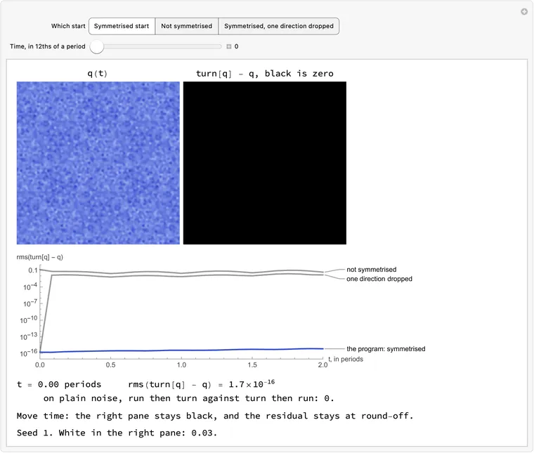
      

      Download ff-turn-why.wl

      The star with the first line and one plane wave without it from the same noise, a table of their T, largest wave's share, turn residual and sweeps, and both rms(lag) curves.
      What this draws, in Wolfram 15.0, 00:05

      20. The loop and the free period

          for sweep in range(1, 400):

      What: the lines below repeat, handing on only , the field, and , the period. One round is called a sweep.

      Why: no single sweep lands. After the first, which wipes the noise, each one moves further from the rest state toward the film, and near the end each cuts what is left to about 0.43 of itself. The limit only stops a failed run: 400 seeds took 30 sweeps at most.

      Try it: drag through the sweeps and watch walk out to the film

      every field is one dot; grey is the film

      q after the free period

      rms(lag) this sweep / last

      What the picture is, and why walks out instead of winding round

      The plane. Take 48 frames of the exact film and find the two directions, in the space of all numbers of a field, along which they spread most: the first two . They hold 46.7% and 46.7% of the film's variance. A field is then a dot: its two coordinates along them (find-film-modes.json, block m6_state_space). The rest state projects onto the plane's centre, within .

      The loop is not a circle. Its radius runs from 18.35 to 25.25 about a mean of 21.93, with period : a rounded triangle. The slide acts on this plane as an exact turn by , which is where the three lobes come from.

      No spiral. Inside a free period the state does go once round. But each sweep is a whole period, and the frames slid back cancel the thirds, so sweep by sweep the dot does not wind. Switch on Also third, two_thirds: those two frames sit and round the loop from , and the slide brings each back beside before the average. Stop a free stretch at instead and the dot flips about each sweep (half_period_free in the same block).

      Not a straight ray either. Seed 1's path happens to be nearly straight. Over seeds 1 to 120, from sweep 2 to the end, the angle turns by a median of 21°, a 90th percentile of 60°, and at most 85.5° (m6b_landings). The thin dashed path in the picture is seed 20, recorded. Where a run lands is steered by the line: the card on return. A caveat on the picture: these two directions were found from the film, so after the turn line nearly all of the noise is out of the plane, 0.0595 against 0.0018 in rms, and the dot cannot show it.

      How many sweeps it takes, and what the limit of 399 is for

      range(1, 400) stops short of 400, so the ceiling is 399 sweeps. The body uses sweep only to report it: nothing depends on the count, and no field or from an earlier sweep is kept.

      Sweeps to land at the program's settings, seeds 5001-5400, each of them on the film (400 of 400; find-film-runs.json):

      sweeps21222324252627282930
      seeds13214491761252451

      The count is explained by one number and one measurement. Late in a run, with , the factor of the slowest mode, and read from the run itself. Then rounded up gives the sweep count on all but one of the first 120 seeds. Each factor of ten in the tolerance costs sweeps (m6b_landings.counts).

      In the first sweeps the lag does not fall, as the chart shows: while the amplitude grows, is not yet meaningful and the lag grows with the field. std() settles at sweep 5 to 10, median 7 (seeds 1-200).

      The limit does its job only where the program is slow or wrong. Without the first line, on the 27 of 400 seeds that reach the film, it takes 312 to 411 sweeps, and 4 of them hit the ceiling a few sweeps short. When it fails has the rest: mostly a raise there does not mean what it says.

      What one sweep costs: of free time and of frames, so ; 1280 + 428 + 428 + 1 calls of rate; every other line takes under a millisecond.

      Mathematica
      (* for sweep in range(1, 400): drag through the sweeps of a real run and watch q walk out to the film's loop, with the field and the lag beside it. About 2 s on an M5. *)
      n = 36; box = 40.;   (* a triangular mesh of n x n nodes, in a repeating box of this side *)
      a = 1.; b = 2.3;     (* the Brusselator's constants; both chemicals diffuse at rate 1 *)
      dt = 0.02;           (* the longest time step *)
      
      (* How fast the chemicals q = {u, v} are changing: diffusion plus reaction. *)
      laplacian[f_] := 2/(3 (box/n)^2) ListCorrelate[{{1, 1, 0}, {1, -6, 1}, {0, 1, 1}}, f, {2, 2}];
      rate[{u_, v_}] := {laplacian[u] + a - (b + 1) u + u^2 v, laplacian[v] + b u - u^2 v};
      
      (* Run time forward by t (fourth-order Runge-Kutta). *)
      simulate[q0_, t_] := Module[{q = q0, steps = Ceiling[t/dt], h, k1, k2, k3, k4},
         h = t/steps;
         Do[
          k1 = rate[q];
          k2 = rate[q + h/2 k1];
          k3 = rate[q + h/2 k2];
          k4 = rate[q + h k3];
          q += h/6 (k1 + 2 k2 + 2 k3 + k4),
          {steps}];
         q];
      
      (* Slide the picture by a third of the box. On the film this costs T/3 of time. *)
      slide[q_] := RotateLeft[q, {0, n/3, 2 n/3}];
      
      (* Turn the picture 120 degrees about the origin. On the film this costs no time. *)
      turn[q_] := Table[f[[Mod[x - y, n] + 1, Mod[-y, n] + 1]], {f, q}, {y, 0, n - 1}, {x, 0, n - 1}];
      
      (* Start from the rest state plus white noise, and find the film. *)
      rest = {ConstantArray[a, {n, n}], ConstantArray[b/a, {n, n}]};
      noise[s_, amp_ : 0.1] := (SeedRandom[s]; rest + RandomVariate[NormalDistribution[0, amp], {2, n, n}]);
      
      (* One run, with every sweep recorded: findFilm's lines, plus the record. *)
      loopRun[q0_] := Module[{q, T = 6.355, third, twoThirds, lag, speed, rows = {}},
         q = (q0 + turn[q0] + turn[turn[q0]])/3;
         Do[
          q = simulate[q, T];
          third = simulate[q, T/3];
          twoThirds = simulate[third, T/3];
          lag = slide[third] - q;
          AppendTo[rows, <|"q" -> q, "third" -> third, "twoThirds" -> twoThirds, "T" -> T, "rms" -> RootMeanSquare[Flatten[lag]]|>];
          If[RootMeanSquare[Flatten[lag]] < 1*^-10, Break[]];
          speed = rate[q];
          T -= Clip[3 Total[lag speed, 3]/Total[speed speed, 3], {-0.1, 0.1}];
          q = (q + slide[third] + slide[slide[twoThirds]])/3,
          {399}];
         rows];
      loopSeed = 1;
      loopRows = loopRun[noise[loopSeed]];
      
      (* The plane: the first two principal components of 48 frames of the film. A field is then one dot. *)
      loopFilm = NestList[simulate[#, loopRows[[-1, "T"]]/48] &, loopRows[[-1, "q"]], 48];
      loopMean = Mean[Flatten /@ Most[loopFilm]];
      loopAxes = Transpose[Last[SingularValueDecomposition[(Flatten[#] - loopMean) & /@ Most[loopFilm], 2]]];
      loopDot[q_] := loopAxes . (Flatten[q] - loopMean);
      loopLoop = loopDot /@ loopFilm;
      loopRange = MinMax[loopFilm[[All, 1]]];
      loopBlue = RGBColor[0.19, 0.29, 0.8];
      
      (* Four points a mesh step, linear on the mesh's own triangles, as the page paints: a turned field then draws as the turned picture. *)
      meshTent = Table[Max[0., 1. - Max[Abs[i], Abs[j], Abs[i - j]]/4.], {j, -3, 3}, {i, -3, 3}];
      meshFine[f_] := ListCorrelate[meshTent, KroneckerProduct[f, Normal[SparseArray[{{1, 1} -> 1.}, {4, 4}]]], {4, 4}];
      
      (* A field on the plane, as a picture: the mesh's two axes are 120 degrees apart. Blue is lo, white is hi. *)
      picture[u_, {lo_, hi_}, size_ : 240] := Colorize[
         Quiet[    (* Wolfram 15's ImageTransformation trips on the notebook's light/dark background, harmlessly *)
          ImageTransformation[Image[Rescale[Reverse[meshFine[u]], {lo, hi}]],
           {#[[1]] + #[[2]]/Sqrt[3.], 2 #[[2]]/Sqrt[3.]}/box + 0.5/(4 n) &, {size, size},
           DataRange -> {{0, 1}, {0, 1}}, PlotRange -> {{-40., 40.}, {-40., 40.}},
           Padding -> "Periodic", Resampling -> "Linear"],
          RemoveAlphaChannel::imginv],
         ColorFunction -> (Blend[{RGBColor[0.118, 0.165, 0.51], RGBColor[0.251, 0.329, 0.808], RGBColor[0.588, 0.667, 0.941], RGBColor[0.961, 0.973, 1.]}, #] &), ColorFunctionScaling -> False];
      
      loopPlane[s_, show_] := With[{path = loopDot[#["q"]] & /@ loopRows, third = loopDot[loopRows[[s, "third"]]], two = loopDot[loopRows[[s, "twoThirds"]]]},
         Graphics[{
           {GrayLevel[0.7], Thickness[0.008], Line[loopLoop]},
           {GrayLevel[0.3], Text["+", loopDot[rest]], Text["rest state", loopDot[rest] + {0, -2.2}]},
           {loopBlue, Dashed, Line[path[[s ;;]]]},
           {loopBlue, Thick, Line[path[[;; s]]], PointSize[0.012], Point[path[[;; s]]]},
           {Darker[Orange], PointSize[0.028], Point[path[[s]]]},
           If[show === "q only", {}, {Black, PointSize[0.018], Point[{third, two}], Text["third", 0.8 third], Text["two_thirds", 0.8 two]}]},
          PlotRange -> 30, ImageSize -> 310]];
      
      loopChart[s_] := With[{m = Length[loopRows]},
         ListLogPlot[{loopRows[[All, "rms"]], loopRows[[All, "rms"]], ConstantArray[1*^-10, m]}, Joined -> {True, False, True},
          PlotStyle -> {loopBlue, Directive[loopBlue, PointSize[0.008]], Directive[Gray, Dashed]}, PlotRange -> {1*^-11, 1}, GridLines -> {{{s, Directive[Orange, Thick]}}, None},
          AxesLabel -> {"sweep", "rms(lag); dashed: tol"}, ImageSize -> {625, 170}, AspectRatio -> Full]];
      
      loopSay[s_] := Module[{dot = loopDot[loopRows[[s, "q"]]], edge},
         edge = First[MaximalBy[loopLoop, Normalize[#] . Normalize[dot] &]];
         Which[
          s == Length[loopRows], "Stop: rms(lag) is under tol. This q, this T and the sweep number are returned.",
          Norm[dot] < 0.97 Norm[edge], "Still inside the loop: the pattern is growing, and the lag rises and falls with it.",
          True, "On the loop now. From here only what is left of the error shrinks, and the lag falls with it."]];
      
      loopView[wanted_, show_] := With[{s = Clip[wanted, {1, Length[loopRows]}]},
         Column[{
           Row[{loopPlane[s, show], Show[picture[loopRows[[s, "q", 1]], loopRange, 480], ImageSize -> 310]}, " "],
           loopChart[s],
           Style[Row[{"Sweep ", s, " of ", Length[loopRows], ", seed ", loopSeed, ".   T = ", NumberForm[loopRows[[s, "T"]], {5, 4}],
              "   rms(lag) = ", ScientificForm[loopRows[[s, "rms"]], 2],
              If[s > 1, Row[{"   this sweep / last = ", NumberForm[loopRows[[s, "rms"]]/loopRows[[s - 1, "rms"]], {3, 2}]}], ""]}], "Text", 13],
           Pane[TextCell[loopSay[s], "Text", FontSize -> 13], 625],
           Pane[TextCell["Field colour: the film's range for u, so the first sweeps look flat.", "Text", FontSize -> 12, FontColor -> Gray], 625]}]];
      
      Manipulate[loopView[s, show],
       {{s, 8, "Sweep"}, 1, Dynamic[Length[loopRows]], 1},
       {{show, "q only", "On the loop"}, {"q only", "also third, two_thirds"}},
       Button["New noise, run it", loopRows = loopRun[noise[++loopSeed]]; s = Length[loopRows], Method -> "Queued"],
       TrackedSymbols :> {s, show, loopRows}, SaveDefinitions -> True]
      

      Download ff-loop.wl

      The film as a closed grey loop with a blue path of dots walking out from the rest state to it, the field beside it, and the lag against sweep below, with a sweep slider.
      What this draws, in Wolfram 15.0, 00:02
      q = simulate(q, T)                          # one free period: what decays, decays

      What: the field runs forward by one whole period . Nothing along the way is kept; on the film it would come back to where it started.

      Why: what the film does not need dies here by itself: one period of diffusion wipes the fine grain of the noise, which the average below would only cut to about a third. The catch is that a few things grow, and the average has to deal with those.

      Try it: drag the time back and forth and watch which bars die

      Near rest: why each wave has its own rate, and which ones grow

      While the field is small, plus the conjugate, with the rest state and the eigenvector of the reaction's Jacobian for . The mesh's six-neighbour stencil has the eigenvalue, for the wave with indices , and the distance between neighbours,

      and because both chemicals each wave only gets its own growth, with the same clock :

      So one period multiplies by . The bars measure this on the real field: , with the left eigenvector, Fourier transformed. Group by , seed 1 from to (find-film-extra-cardsB.json, find_film_extra_cardsB.py):

      shellindiceslaw, per period
      010.15002.594
      260.11722.106
      660.05211.392
      860.01971.134
      1412-0.07620.616
      186-0.13940.412

      Only 19 of the 1296 indices grow. The finest shrink by by the law, since reaches -4.86.

      Where the law does not hold. The small orange ticks are the law. The first bar, the field's mean, stops short of its tick: 1.70 against 2.59. And the finest band ends at , not the it would reach on its own. The natural suspect is the reaction's quadratic and cubic terms, which feed the mean and the fine waves from what is left of the noise. The test: at noise amplitude instead of , those two numbers are the second of each pair above: the mean's ratio is 2.585, on the law, and the finest band falls as far as the law says.

      In rms over all the field: the first free period takes std() from 0.0595 to 0.0133 on seed 1. Seen in the film's plane (the card on the loop), what lies out of the plane falls from 0.0595 to 0.0139, and 0.0077 of that is the rest state's own distance from the plane, not noise. So one period cuts the noise hard, and does not remove it.

      On the film: a period multiplies each mode by

      Near the end of a run, is close to the film and a small difference evolves linearly. Let be simulate for time , the slide, and linearised at the exact frame, with eigenvalues . commutes with exactly (m2_commute) and , so : a free period multiplies a mode by . The bars are the leading modes of the turn-symmetric fields, from find-film-modes.json, block m3_spectrum; the dense matrix agrees with them.

      mode, a free periodthe average aloneboth, one sweep
      unison1.16080.03030.0351
      time shift1.00001.00001.0000
      slow0.52350.81850.4284

      Read across. The unison mode grows in the free period and the average takes nearly all of it. The time shift, a frame further along the film, is untouched by either. The slow mode is the one the free period earns its keep on: the average leaves 0.82 of it, and the free period brings that to 0.43. That is most of why 26 sweeps suffice against 107 without it (how many free periods).

      The experiment on screen. Start from the exact frame plus of the unison mode and of the slow mode, really simulate, and subtract the frame. The slow part dies, so the picture settles into the unison mode's own shape, and from then on the factor per period rises to 1.16, itself. Over a long run from a returned frame the rms averages 1.152, a little under, because the mode's real part also turns as it grows (after_return.turning; the card on what the frame cannot do).

      Where the comment oversimplifies. "What decays, decays" leaves out what grows. Near rest 19 indices grow by up to 2.59 a period, and that is wanted, since the film has to grow out of them. On the film the unison mode grows 1.16, which is not. Also, the free run is not quite the same arithmetic as three thirds: 320 RK4 steps against 107 three times, so the exact frame comes back to by this line and to by three thirds. It is what sets how small the lag can get: the card on when to stop.

      Mathematica
      (* q = simulate(q, T): drag the time and watch which bars die. Near rest, one bar per wave size, measured from the real field as the noise dies. On the film, one bar per mode, beside a real push. Runs the program and finds the modes live. About 5 s on an M5. *)
      n = 36; box = 40.;   (* a triangular mesh of n x n nodes, in a repeating box of this side *)
      a = 1.; b = 2.3;     (* the Brusselator's constants; both chemicals diffuse at rate 1 *)
      dt = 0.02;           (* the longest time step *)
      
      (* How fast the chemicals q = {u, v} are changing: diffusion plus reaction. *)
      laplacian[f_] := 2/(3 (box/n)^2) ListCorrelate[{{1, 1, 0}, {1, -6, 1}, {0, 1, 1}}, f, {2, 2}];
      rate[{u_, v_}] := {laplacian[u] + a - (b + 1) u + u^2 v, laplacian[v] + b u - u^2 v};
      
      (* Run time forward by t (fourth-order Runge-Kutta). *)
      simulate[q0_, t_] := Module[{q = q0, steps = Ceiling[t/dt], h, k1, k2, k3, k4},
         h = t/steps;
         Do[
          k1 = rate[q];
          k2 = rate[q + h/2 k1];
          k3 = rate[q + h/2 k2];
          k4 = rate[q + h k3];
          q += h/6 (k1 + 2 k2 + 2 k3 + k4),
          {steps}];
         q];
      
      (* Slide the picture by a third of the box. On the film this costs T/3 of time. *)
      slide[q_] := RotateLeft[q, {0, n/3, 2 n/3}];
      
      (* Turn the picture 120 degrees about the origin. On the film this costs no time. *)
      turn[q_] := Table[f[[Mod[x - y, n] + 1, Mod[-y, n] + 1]], {f, q}, {y, 0, n - 1}, {x, 0, n - 1}];
      
      (* One frame of the film, its period T, and the number of sweeps it took. *)
      findFilm[q0_, T0_ : 6.355, tol_ : 1*^-10] := Module[{q, T = T0, third, twoThirds, lag, speed},
         q = (q0 + turn[q0] + turn[turn[q0]])/3;    (* costs no time, so impose it once and it stays *)
         Do[
          q = simulate[q, T];                       (* one free period: what decays, decays *)
          third = simulate[q, T/3];
          twoThirds = simulate[third, T/3];
      
          lag = slide[third] - q;                   (* zero on the film *)
          If[RootMeanSquare[Flatten[lag]] < tol, Return[{q, T, sweep}, Module]];
      
          (* T is off by 3 x lag / speed. Move it gently, since at first it's all noise. *)
          speed = rate[q];
          T -= Clip[3 Total[lag speed, 3]/Total[speed speed, 3], {-0.1, 0.1}];
      
          (* What obeys the rule survives the average; what ticks in unison cancels. *)
          q = (q + slide[third] + slide[slide[twoThirds]])/3,
          {sweep, 399}];
         $Failed];
      
      (* Start from the rest state plus white noise, and find the film. *)
      rest = {ConstantArray[a, {n, n}], ConstantArray[b/a, {n, n}]};
      noise[s_, amp_ : 0.1] := (SeedRandom[s]; rest + RandomVariate[NormalDistribution[0, amp], {2, n, n}]);
      
      (* Near rest. A = l . (q - rest), with l the left eigenvector of the reaction's Jacobian for sigma + i omega, Fourier transformed: one size for each band of wave sizes. *)
      freeJ = {{b - 1, a^2}, {-b, -a^2}};
      freeLeft = First[Pick[Eigenvectors[Transpose[freeJ]], Im[Eigenvalues[Transpose[freeJ]]], v_ /; v > 0]];
      freeSigma = (b - 1 - a^2)/2;
      freeShell = Table[With[{m = Mod[i + n/2, n] - n/2, k = Mod[j + n/2, n] - n/2}, m^2 + k^2 + (m + k)^2], {j, 0, n - 1}, {i, 0, n - 1}];
      freeBands = {{0, 0}, {2, 2}, {6, 6}, {8, 8}, {14, 14}, {18, 18}, {24, 26}, {32, 62}, {64, 200}, {202, 800}, {802, 100000}};
      freeWhere = Function[band, Position[freeShell, s_ /; band[[1]] <= s <= band[[2]]]] /@ freeBands;
      freeSizes[q_] := With[{hat = Abs[Fourier[freeLeft . (q - rest)]]^2}, Sqrt[Mean[Extract[hat, #]]] & /@ freeWhere];
      
      (* The first free period: the turn line on noise, then 16 pieces of T0 = 6.355. *)
      freeT0 = 6.355;
      freeRest = NestList[simulate[#, freeT0/16] &, With[{q0 = noise[1]}, (q0 + turn[q0] + turn[turn[q0]])/3], 16];
      freeRestSizes = freeSizes /@ freeRest;
      
      (* The linear law for the six coarsest bands: a wave (m, k) grows as Exp[(sigma + Lambda) t]. *)
      freeLambda[{m_, k_}] := 2/(3 (box/n)^2) (2 Cos[2 Pi m/n] + 2 Cos[2 Pi k/n] + 2 Cos[2 Pi (m + k)/n] - 6);
      freeLaw[t_] := Exp[(freeSigma + freeLambda[#]) t] & /@ {{0, 0}, {1, 0}, {1, 1}, {2, 0}, {2, 1}, {3, 0}};
      
      (* Four points a mesh step, linear on the mesh's own triangles, as the page paints: a turned field then draws as the turned picture. *)
      meshTent = Table[Max[0., 1. - Max[Abs[i], Abs[j], Abs[i - j]]/4.], {j, -3, 3}, {i, -3, 3}];
      meshFine[f_] := ListCorrelate[meshTent, KroneckerProduct[f, Normal[SparseArray[{{1, 1} -> 1.}, {4, 4}]]], {4, 4}];
      
      (* A field on the plane, as a picture: the mesh's two axes are 120 degrees apart. Blue is lo, white is hi. *)
      picture[u_, {lo_, hi_}, size_ : 240] := Colorize[
         Quiet[    (* Wolfram 15's ImageTransformation trips on the notebook's light/dark background, harmlessly *)
          ImageTransformation[Image[Rescale[Reverse[meshFine[u]], {lo, hi}]],
           {#[[1]] + #[[2]]/Sqrt[3.], 2 #[[2]]/Sqrt[3.]}/box + 0.5/(4 n) &, {size, size},
           DataRange -> {{0, 1}, {0, 1}}, PlotRange -> {{-40., 40.}, {-40., 40.}},
           Padding -> "Periodic", Resampling -> "Linear"],
          RemoveAlphaChannel::imginv],
         ColorFunction -> (Blend[{RGBColor[0.118, 0.165, 0.51], RGBColor[0.251, 0.329, 0.808], RGBColor[0.588, 0.667, 0.941], RGBColor[0.961, 0.973, 1.]}, #] &), ColorFunctionScaling -> False];
      
      (* Bars up or down from a line at 1, on a log axis, with a floor. *)
      freeBars[values_, colors_, floor_, ticks_] := Graphics[{
          MapThread[{#3, Rectangle[{#1 - 0.38, 0}, {#1 + 0.38, Log10[Clip[#2, {floor, 10}]]}]} &, {Range[Length[values]], values, colors}],
          {Black, Line[{{0.4, 0}, {Length[values] + 0.6, 0}}]}, ticks},
         PlotRange -> {{0.4, Length[values] + 0.6}, {Log10[floor], 0.8}}, AspectRatio -> 1, ImageSize -> 310, Frame -> {{True, False}, {False, False}},
         FrameTicks -> {{Table[{e, Superscript[10, e]}, {e, Ceiling[Log10[floor]], 0}], None}, {None, None}}];
      
      freeRestView[j_] := With[{ratio = freeRestSizes[[j + 1]]/First[freeRestSizes], t = j freeT0/16},
         Column[{
           Row[{Labeled[Show[picture[freeRest[[j + 1, 1]], {0.85, 1.15}, 480], ImageSize -> 310], Style["q at this moment", "Text", 13], Top],
             Labeled[freeBars[ratio, If[# >= 1, RGBColor[0.19, 0.29, 0.8], GrayLevel[0.7]] & /@ ratio, 1*^-5,
               {Darker[Orange], Thick, MapIndexed[Line[{{First[#2] - 0.5, Log10[#1]}, {First[#2] + 0.5, Log10[#1]}}] &, freeLaw[t]],
                Black, Text["coarse", {1.2, 0.65}], Text["fine", {10.8, 0.65}]}], Style["each wave size, against its start", "Text", 13], Top]}, " "],
           Style[Row[{"t = ", j, "/16 of a period.   std(u) = ", NumberForm[StandardDeviation[Flatten[freeRest[[j + 1, 1]]]], {5, 4}], "   finest waves x ", ScientificForm[Last[ratio], 2]}], "Text", 13],
           Pane[TextCell[Which[
              j == 0, "White noise: every wave size is present, and all the bars start at 1.",
              j < 16, "The finest waves go first: the bars at the right drop while the coarse ones hold.",
              True, "After one period: the grain is gone, and " <> ToString[Count[ratio, v_ /; v > 1]] <> " of " <> ToString[Length[ratio]] <> " sizes have grown. What is left is what the film can grow from."], "Text", FontSize -> 13], 625],
           Pane[TextCell["The first sweep: seed 1 after the turn line, really simulated. Blue grew, grey shrank; a bar that reaches the floor went lower. Orange ticks: the linear law. Field colour: u from 0.85 to 1.15.", "Text", FontSize -> 12, FontColor -> Gray], 625]}]];
      
      (* On the film. The leading modes of M = slide after simulate[., T/3], by Arnoldi on turn-symmetric fields, each product with M by a finite difference. A free period multiplies a mode by |mu|^3. *)
      {freeQ, freeT, freeSweeps} = findFilm[noise[1]];
      freeM[v_] := With[{e = 1*^-5, x = ArrayReshape[v, {2, n, n}]},
         With[{w = slide[simulate[freeQ + e x, freeT/3] - simulate[freeQ - e x, freeT/3]]/(2 e)}, Flatten[(w + turn[w] + turn[turn[w]])/3]]];    (* kept to the turn-symmetric fields *)
      freeArnoldi[v0_, m_] := Module[{basis = {Normalize[v0]}, hess = ConstantArray[0., {m + 1, m}], w},
         Do[
          w = freeM[basis[[j]]];
          Do[hess[[i, j]] = basis[[i]] . w; w -= hess[[i, j]] basis[[i]], {i, j}];
          hess[[j + 1, j]] = Norm[w];
          AppendTo[basis, w/hess[[j + 1, j]]],
          {j, m}];
         {basis[[;; m]], hess[[;; m, ;; m]]}];
      {freeBasis, freeHess} = freeArnoldi[Flatten[With[{r = noise[2] - rest}, r + turn[r] + turn[turn[r]]]], 60];
      {freeMu, freeRitz} = Eigensystem[freeHess];
      freeOrder = Ordering[Abs[freeMu], All, Greater];
      {freeMu, freeRitz} = {freeMu[[freeOrder]], freeRitz[[freeOrder]]};
      freeMode[i_] := With[{x = Re[freeRitz[[i]] . freeBasis]}, ArrayReshape[x/RootMeanSquare[x], {2, n, n}]];    (* the real part, unit rms *)
      freeSlowAt = First[FirstPosition[freeMu, v_ /; Im[v] == 0 && Re[v] > 0 && Abs[v] < 0.95]];    (* the largest that shrinks, and doesn't tick *)
      
      (* The experiment: the frame plus a small push of two modes, really simulated, minus the frame. *)
      freeKicked = NestList[simulate[#, freeT] &, freeQ + 1*^-3 (freeMode[1] + freeMode[freeSlowAt]), 8];
      freePush = (# - freeQ) & /@ freeKicked;
      freeShown = DeleteDuplicatesBy[Abs[freeMu], Round[#, 1*^-5] &][[;; 14]]^3;
      freeWhite = 0.008;
      
      freeGrey[u_] := Quiet[
         ImageTransformation[Image[Clip[Abs[Reverse[meshFine[u]]]/freeWhite, {0, 1}]],
          {#[[1]] + #[[2]]/Sqrt[3.], 2 #[[2]]/Sqrt[3.]}/box + 0.5/(4 n) &, {480, 480},
          DataRange -> {{0, 1}, {0, 1}}, PlotRange -> {{-40., 40.}, {-40., 40.}},
          Padding -> "Periodic", Resampling -> "Linear"],
         RemoveAlphaChannel::imginv];
      
      freeFilmView[k_] := With[{bars = freeShown^k},
         Column[{
           Row[{Labeled[Show[freeGrey[freePush[[k + 1, 1]]], ImageSize -> 310], Style["a small push: size, black is zero", "Text", 13], Top],
             Labeled[freeBars[bars, ReplacePart[ConstantArray[GrayLevel[0.7], 14], {1 -> Darker[Orange], First[FirstPosition[Round[freeShown, 1*^-3], Round[Abs[freeMu[[freeSlowAt]]]^3, 1*^-3]]] -> RGBColor[0.19, 0.29, 0.8]}], 1*^-3, {}], Style["each mode of the film, against its start", "Text", 13], Top]}, " "],
           Style[Row[{"After ", k, " free periods.   rms(push) = ", ScientificForm[RootMeanSquare[Flatten[freePush[[k + 1]]]], 2], "   unison bar x ", NumberForm[bars[[1]], {3, 2}]}], "Text", 13],
           Pane[TextCell[Which[
              k == 0, "The push is a mix of two modes, and every bar starts at 1.",
              k < 3, "The slow mode and everything below it shrink. The unison bar rises above the line.",
              True, "What is left of the push is the unison mode, and it keeps growing. A free period alone never ends on the film: that is what the average is for."], "Text", FontSize -> 13], 625],
           Pane[TextCell["The last sweeps: the frame plus 0.001 of two modes, really simulated, minus the frame. White: 0.008. Bars: what one free period does to each mode. Orange: the unison mode; next, on the line, the time shift, a frame a little later, which is still the film. Blue: the slow mode, the largest that shrinks.", "Text", FontSize -> 12, FontColor -> Gray], 625]}]];
      
      TabView[{
        "Near rest" -> Manipulate[freeRestView[j], {{j, 16, "Time, in 16ths of a period"}, 0, 16, 1, Appearance -> "Labeled"}, SaveDefinitions -> True],
        "On the film" -> Manipulate[freeFilmView[k], {{k, 1, "After, in free periods"}, 0, 8, 1, Appearance -> "Labeled"}, SaveDefinitions -> True]}]
      

      Download ff-free.wl

      Near rest: the field after one free period beside one bar per wave size, up or down from a line at 1, the fine ones falling furthest, with orange ticks for the linear law and a time slider.
      What this draws, in Wolfram 15.0, 00:05
      q = simulate(q, T)                          # one free period: what decays, decays

      What: the program spends exactly one free period per sweep. Call the number . Nothing forces : the same code runs with any .

      Why: too few and the run needs many more sweeps; too many and each sweep costs more, and past about half the runs and more end on no film at all. is far from that edge and close to the cheapest.

      Try it: move , then run it live

      what a landing costs: periods simulated in all

      how many runs land on the film

      Dashed: where the overtakes the star.

      on the film sweeps periods

      Medians from the table of fresh seeds at noise , over the runs that landed.

      Why not none: what a free period buys

      Near the film a sweep multiplies a mode by : free periods, then the two frames and the average (the factor is the card on both lines together). The largest of these over all modes but the neutral time shift sets the rate, and each sweep costs periods. From the spectrum (find-film-extra-cardsB.json, block cost_by_k), against the runs (find-film-runs.json, block free_periods, seeds 1-40):

      leading factorwhich modesweeps, predictedsweeps, runperiods, run
      00.818slow mode108.810771.3
      10.428slow mode25.72643.3
      20.224slow mode14.61540.0
      30.117slow mode10.21140.3
      40.061slow mode7.81256.0
      60.074unison8.413.590.0

      Prediction: , with the row's leading factor and the constant in , the program's median at . It works up to . From it runs low, since a landing also has to grow out of the noise, and that takes sweeps however fast the end is; the fit knows only the end.

      So works, on every seed, and costs 71.3 periods to the program's 43.3. The average alone can do the whole job; it does it slowly, because its factor on the slow mode is 0.82 and it costs only of a period. And or is a little cheaper than the program's : 40.0 and 40.3 periods. The program does not take the cheapest . Its comment names one, and it has more margin; the difference is under a tenth. All these rows use three frames; with other numbers of frames the costs shift (frames_grid; the average's filter).

      Nor must the free stretch be a whole period. Run simulate(q, x * T) for other , the rest of the program unchanged: every run lands on the film. A whole period is what keeps each sweep's start in one place on the loop (the card on the loop), and it is near the cheapest; it is not what makes the method work. Four seeds each, seeds 1-4, so a check and not a table (find-film-extra-fix4.json, find_film_extra_fix4.py):

      on the filmmedian sweepsperiods
      4 of 460.055.0
      4 of 452.552.5
      4 of 442.049.0
      4 of 426.043.3
      4 of 419.542.3
      Why not many: the uniform mode wins a race near rest, long before the unison mode's limit

      The first guess is the unison mode, the one that grows 1.16 a period on the film. That sets a limit only for a run already on the film. From the exact film with a kick, the program holds up to and fails at 24, exactly where crosses 1, at (free_periods_from_film, unison_k).

      From noise it breaks far sooner, at about 8 to 9, at any noise amplitude. The reason lies near rest, before there is any film. The uniform mode grows a period and the three waves of the pattern . The average cuts the uniform mode more, so per sweep it starts behind: the ratio uniform to star is 0.197 at , and every extra free period multiplies it by . It crosses 1 at . Real sweeps at : uniform ×527.9, star ×505.9.

      The test, runs that land on the film from clean starts at amplitude per wave, 10 seeds each, and from noise with the field's mean reset to rest after each free period until the pattern is big, 30 seeds each (free_periods_why):

      star alonestar + uniformstar + noise, mean removed
      810101030
      101011021
      12100810
      1610001
      2010000

      A clean star holds to . Add the uniform mode and it fails from . So uniform growth is the first cause. The cut waves come in past about , when the average can no longer take them down fast enough: that part rests on these clean starts, not on following a run through a free period.

      A warning about how it fails. Past the limit most runs do not raise. walks to near or under 0, and the program returns with no error. The rest go nearly uniform and raise at sweep 399. Press Run this live at to see one (when it fails).

      The first table, seeds 1-40

      " near 0" returned with no error. The sliders above use a second table on fresh seeds, finer in (free_periods_fresh); where the two meet the share on the film agrees. From their medians do not: this table counts whatever returned, the sliders only the runs on the film.

      film near 0raisedsweepsperiods
      040/4000107.071.3
      140/400026.043.3
      240/400015.040.0
      340/400011.040.3
      440/400012.056.0
      637/403013.590.0
      824/4015124.0208.0
      121/40271277.0975.3
      160/40221879.01316.7

      Where a row is mostly failures, its sweeps and periods are medians over whatever returned, so they say little.

      Mathematica
      (* q = simulate(q, T) in each sweep: how many free periods? Move k along the table measured over fresh seeds, then run that k live. The real program at k = 1 runs on evaluation. About 2 s on an M5; a live run of a k past the safe range can take minutes. *)
      n = 36; box = 40.;   (* a triangular mesh of n x n nodes, in a repeating box of this side *)
      a = 1.; b = 2.3;     (* the Brusselator's constants; both chemicals diffuse at rate 1 *)
      dt = 0.02;           (* the longest time step *)
      
      (* How fast the chemicals q = {u, v} are changing: diffusion plus reaction. *)
      laplacian[f_] := 2/(3 (box/n)^2) ListCorrelate[{{1, 1, 0}, {1, -6, 1}, {0, 1, 1}}, f, {2, 2}];
      rate[{u_, v_}] := {laplacian[u] + a - (b + 1) u + u^2 v, laplacian[v] + b u - u^2 v};
      
      (* Run time forward by t (fourth-order Runge-Kutta). *)
      simulate[q0_, t_] := Module[{q = q0, steps = Ceiling[t/dt], h, k1, k2, k3, k4},
         h = t/steps;
         Do[
          k1 = rate[q];
          k2 = rate[q + h/2 k1];
          k3 = rate[q + h/2 k2];
          k4 = rate[q + h k3];
          q += h/6 (k1 + 2 k2 + 2 k3 + k4),
          {steps}];
         q];
      
      (* Slide the picture by a third of the box. On the film this costs T/3 of time. *)
      slide[q_] := RotateLeft[q, {0, n/3, 2 n/3}];
      
      (* Turn the picture 120 degrees about the origin. On the film this costs no time. *)
      turn[q_] := Table[f[[Mod[x - y, n] + 1, Mod[-y, n] + 1]], {f, q}, {y, 0, n - 1}, {x, 0, n - 1}];
      
      (* Start from the rest state plus white noise, and find the film. *)
      rest = {ConstantArray[a, {n, n}], ConstantArray[b/a, {n, n}]};
      noise[s_, amp_ : 0.1] := (SeedRandom[s]; rest + RandomVariate[NormalDistribution[0, amp], {2, n, n}]);
      
      (* Typed, measured with the page's Python at noise 0.1, seeds 8001-8060 for k up to 3 and 8101-8130 above:
         {k, runs on the film, runs, median sweeps, median periods simulated}; the medians are over the runs on the film. *)
      fcTable = {{0, 60, 60, 106, 70.67}, {1, 60, 60, 26, 43.33}, {2, 60, 60, 15, 40.0}, {3, 60, 60, 11, 40.33},
         {4, 30, 30, 12, 56.0}, {5, 30, 30, 13, 73.67}, {6, 29, 30, 14, 93.33}, {7, 26, 30, 15, 115.0},
         {8, 21, 30, 18, 156.0}, {9, 13, 30, 19, 183.7}, {10, 4, 30, 18, 192.0}, {12, 1, 30, 16, 202.7}};
      fcCross = 7.796;    (* where the uniform mode overtakes the three waves: growth 2.5941 against 2.1058 a period, near rest *)
      
      (* findFilm's lines with k free periods in place of one. Past the safe range T can walk to 0, where simulate would divide by zero: that ends the run too. *)
      fcRun[s_, k_] := Module[{q0 = noise[s], q, T = 6.355, third, twoThirds, lag, speed, sweeps = 0, status = "raised"},
         q = (q0 + turn[q0] + turn[turn[q0]])/3;
         Do[
          sweeps = i;
          If[T <= 0, status = "T reached 0"; Break[]];
          q = Nest[simulate[#, T] &, q, k];
          third = simulate[q, T/3];
          twoThirds = simulate[third, T/3];
          lag = slide[third] - q;
          If[RootMeanSquare[Flatten[lag]] < 1*^-10, status = "returned"; Break[]];
          speed = rate[q];
          T -= Clip[3 Total[lag speed, 3]/Total[speed speed, 3], {-0.1, 0.1}];
          q = (q + slide[third] + slide[slide[twoThirds]])/3,
          {i, 399}];
         <|"k" -> k, "seed" -> s, "sweeps" -> sweeps, "status" -> status, "T" -> T, "std" -> StandardDeviation[Flatten[q[[1]]]]|>];
      
      (* What became of a run, in words. *)
      fcNum[x_] := ToString[NumberForm[x, 3, ExponentFunction -> (Null &)]];
      fcKind[r_] := Which[
         r["status"] === "raised", "no convergence: the program raises, std(u) " <> fcNum[r["std"]] <> ".",
         Abs[r["T"]] < 1*^-3 || r["status"] === "T reached 0", "T near 0 and a nearly uniform field, std(u) " <> fcNum[r["std"]] <> ", returned with no error.",
         Abs[r["T"] - 6.3901599] < 1*^-6 && r["std"] > 0.2, "the film: T = " <> ToString[NumberForm[r["T"], 8]] <> ", std(u) " <> fcNum[r["std"]] <> ".",
         True, "T = " <> ToString[NumberForm[r["T"], 5]] <> ", std(u) " <> fcNum[r["std"]] <> "."];
      fcReport[r_] := "Live, k = " <> ToString[r["k"]] <> ", seed " <> ToString[r["seed"]] <> ": after " <> ToString[r["sweeps"]] <> " sweeps, " <> fcKind[r];
      fcSeed = 1;
      fcLive = fcReport[fcRun[fcSeed, 1]];
      
      fcPlot[values_, k_, label_, range_, extra_] := ListLinePlot[Transpose[{fcTable[[All, 1]], values}], Mesh -> All, MeshStyle -> PointSize[0.012], PlotRange -> {{0, 12}, range}, ImageSize -> {620, 170}, AspectRatio -> Full,
         PlotStyle -> RGBColor[0.19, 0.29, 0.8], GridLines -> {{{k, Directive[Orange, Thick]}}, None}, AxesLabel -> {"k", label}, Epilog -> extra];
      
      fcSay[k_] := Which[
         k == 0, "No free period: it still lands, every time, but takes 106 sweeps against 26. Those sweeps are cheap, and the total still comes to more.",
         k == 1, "The program: safe by a wide margin, and close to the cheapest.",
         k <= 3, "Slightly cheaper than the program: fewer sweeps, each costing more.",
         k <= 5, "Still lands, every time, but the bill is rising: the sweep count no longer falls.",
         k <= 9, "Past the safe range: more and more runs end somewhere that is not the film.",
         True, "Nearly nothing lands. Most of these return with T near 0 and no error, so a caller would not know."];
      
      fcView[k_] := With[{row = First[Select[fcTable, #[[1]] == k &]]},
         Column[{
           fcPlot[fcTable[[All, 5]], k, "periods simulated to land", {0, 250}, {Text["the program", {1.5, 95}]}],
           fcPlot[100. fcTable[[All, 2]]/fcTable[[All, 3]], k, "% of runs on the film", {0, 100},
            {Gray, Dashed, Line[{{fcCross, 0}, {fcCross, 100}}], Text["uniform mode overtakes the three waves", {fcCross, 55}, {1.05, 0}]}],
           Style[Row[{"on the film ", row[[2]], " of ", row[[3]], "    sweeps ", row[[4]], "    periods ", row[[5]]}], "Text", 13],
           Pane[TextCell[fcSay[k], "Text", FontSize -> 13], 620]}]];
      
      Manipulate[Column[{fcView[k], Pane[TextCell[fcLive, "Text", FontSize -> 13], 620]}],
       {{k, 1, "Free periods per sweep, k"}, fcTable[[All, 1]], ControlType -> Slider, Appearance -> "Labeled"},
       Button["Run this k live", fcLive = "Running k = " <> ToString[k] <> "..."; fcLive = fcReport[fcRun[++fcSeed, k]], Method -> "Queued"],
       SaveDefinitions -> True]
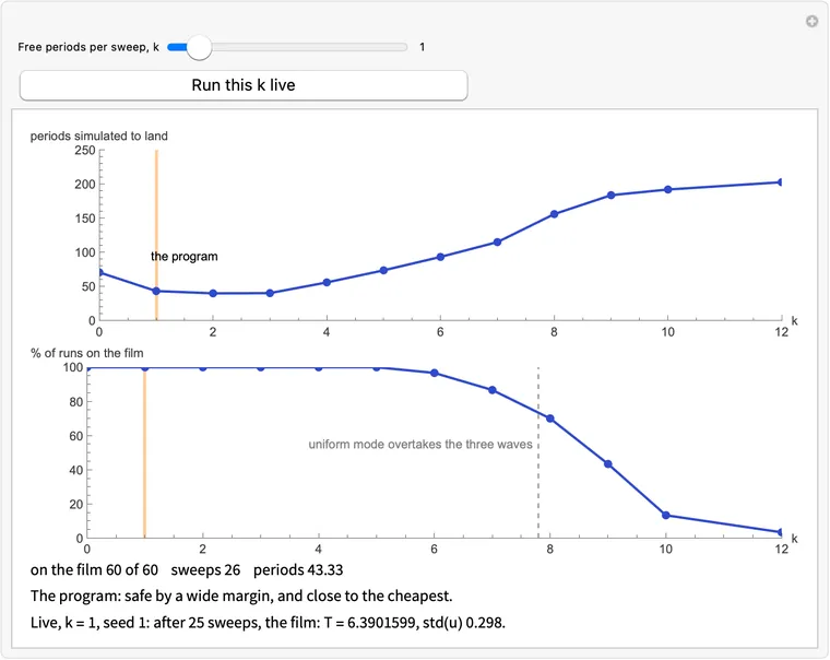
      

      Download ff-free-count.wl

      Periods simulated to land and the share of runs on the film, each against the number of free periods k, with a slider on k and a button that runs that k live.
      What this draws, in Wolfram 15.0, 00:02
          steps = int(np.ceil(t / dt))
          h = t / steps
          for _ in range(steps):
              k1 = rate(q)
              k2 = rate(q + h / 2 * k1)
              k3 = rate(q + h / 2 * k2)
              k4 = rate(q + h * k3)
              q = q + h / 6 * (k1 + 2 * k2 + 2 * k3 + k4)

      What: inside simulate, time is cut into steps equal steps of length . Each step asks rate for the slope four times, and moves by a weighted mean of the four.

      Why: four slopes per step make the time error fall as , so at this cost the film's comes out within . And is set so the last step lands exactly on : the program changes every sweep, and has to ask for that exact time.

      Try it: stretch the step and watch where each slope points

      Four slopes with weights 1, 2, 2, 1: where they come from, and what they buy

      This is the classical fourth-order Runge-Kutta rule. For :

      is the slope where you stand, and two estimates at the midpoint, at the end. If depended only on time the rule would be Simpson's, with weights , the two midpoint estimates sharing the middle weight. Expanding in , the rule agrees with the exact flow through , so one step's error is of order and the error over a fixed time of order . The chart on the right shows the on one cell: halve and the step's error falls by about 32.

      The measured . The film's period found by the program's loop, from the exact frame, with the free period run as three thirds, to a lag under . elsewhere on this page is the film's period at the program's own , not this limit. Against the fourth-order extrapolation (find-film-extra-cardsB.json, block integrators; find_film_extra_cardsB.py):

      methodrate calls per unit timeerror in
      RK40.040100
      RK4, the program0.020200
      RK40.010400
      Heun, two slopes0.010200
      Euler, one slope0.005200

      The program's row, the Heun row and the Euler row cost the same, so read their errors across: that is what four slopes buy. Halving divides RK4's error by 15.6 and then by 16.1, close to the the order predicts. Euler's film is also a different film: its std() is 0.2956 against RK4's 0.2922. The likely reason, an estimate and not a test: one slope turns a rotation at into a spiral with a false growth rate of about , which the reaction has to balance.

      Nothing breaks the symmetries. A step is rate calls and linear combinations, so it commutes with whatever rate commutes with. The slide commutes with simulate to 0, bit for bit; the turn to , where only the order of the additions changes (m2_commute).

      On the picture. A cell with the same chemicals everywhere has a zero Laplacian, so only the reaction is left: the check file holds the cell's arithmetic to rate and simulate on a uniform field. The plane shows the reaction's own closed curve; on the real mesh the same rule runs on numbers at once, with diffusion in the slopes.

      Why ceil, and why is over the steps and not

      dt is the longest step allowed, not the step. changes every sweep, and is not a whole number. So ceil rounds the count up, which keeps , and shrinks the step slightly so that the steps add up to , exactly.

      What happens without it. With left at , every run ends on a multiple of , up to past the time asked for, and the line can no longer steer anything smaller than that. Two seeds, 60 sweeps: the lag never fell below , and ended at 6.3695 and 6.3844, far from the film's (block fixed_h). Most simulations would never notice a time error of one step. A program comparing two frames to cannot live with it, so this one line is essential.

      The side effect. is then not the same for every call. At , simulate(q, T) takes 320 steps and simulate(q, T / 3) takes 107, so three thirds take one step more than the whole, with a slightly different . The two ways of running one period differ by . That small mismatch, not round-off, sets the smallest lag the program can reach: at where the counts agree the floor falls from to (lag_floor_dt; the card on when to stop). Move the slider in the second view: the mismatch is 0, 1 or 2 by .

      How long a step may be, and why is 0.02

      RK4 multiplies a mode with rate by , with . On the negative real axis up to . The stencil's most negative eigenvalue is -4.86, so diffusion alone limits to 0.573. On the film the limit is a little lower: RK4 at a fixed step stays finite for 60 periods at and blows up at (find-film-runs.json, block dt). The program's is well below all of this: nothing here is near unstable.

      What sets is the stop test. Up to every seed lands. Longer steps land only sometimes:

      steps , floor of rms(lag)seeds returned
      0.01640, 64210 of 10
      0.02320, 32110 of 10
      0.04160, 1620 of 10
      0.0880, 810 of 10

      At the film is found and the lag stalls above the program's tolerance, so it raises: is the lag there. Where the two counts happen to agree it lands anyway, at for one: a comb, not an edge (dt.comb; the card on when it fails). So is the longest round step safely under the tolerance, on the seeds tried; nothing here says it is optimal.

      Mathematica
      (* Inside simulate: one uniform cell's four slopes, the error of a step against its length, and the step count that lands on t. Under a second on an M5. *)
      a = 1.; b = 2.3;     (* the Brusselator's constants; both chemicals diffuse at rate 1 *)
      dt = 0.02;           (* the longest time step *)
      
      (* A cell with the same chemicals everywhere: the Laplacian is zero, so rate is the reaction alone. simulate's lines, on it. *)
      rkCell[{u_, v_}] := {a - (b + 1) u + u^2 v, b u - u^2 v};
      rkStep[p_, h_] := Module[{k1, k2, k3, k4},
         k1 = rkCell[p];
         k2 = rkCell[p + h/2 k1];
         k3 = rkCell[p + h/2 k2];
         k4 = rkCell[p + h k3];
         <|"k" -> {k1, k2, k3, k4}, "at" -> {p, p + h/2 k1, p + h/2 k2, p + h k3}, "end" -> p + h/6 (k1 + 2 k2 + 2 k3 + k4)|>];
      rkEnd[p_, h_] := rkStep[p, h]["end"];
      rkExact[p_, t_] := With[{m = Max[4, Ceiling[t/0.002]]}, Nest[rkEnd[#, t/m] &, p, m]];    (* the same rule, far finer *)
      
      (* The cell's closed curve, from a point on it, and where the step starts. *)
      rkCycle = NestList[rkEnd[#, 0.01] &, {1., 2.957924586702392}, 800];
      rkStart = rkCycle[[201]];
      rkLengths = Table[0.02 100^(i/30), {i, 0, 30}];
      
      (* The slopes, each drawn from where it is read, of length h x slope. Solid dot: four slopes. Ring: the exact end. Hollow dot: one slope. *)
      rkPlane[p_, h_] := With[{s = rkStep[p, h], euler = p + h rkCell[p], exact = rkExact[p, h], blue = RGBColor[0.19, 0.29, 0.8]},
         Graphics[{
           {GrayLevel[0.7], Thickness[0.008], Line[rkCycle]},
           {Darker[Orange], Thick, Line[NestList[rkEnd[#, h/40] &, p, 40]]},
           MapThread[{blue, Arrow[{#1, #1 + h #2}], PointSize[0.012], Point[#1], Text[#3, #1 + h #2, {-1.2, 0}]} &, {s["at"], s["k"], {"k1", "k2", "k3", "k4"}}],
           {Black, PointSize[0.022], Point[s["end"]], Circle[euler, 0.03], Text["Euler", euler, {0, 1.6}]},
           {Darker[Orange], Thick, Circle[exact, 0.055]}},
          PlotRange -> {{0.25, 2.35}, {0.95, 3.45}}, Frame -> True, FrameLabel -> {"u", "v"}, ImageSize -> 310]];
      
      (* The error of one step against h, on log axes: four slopes against one. Remembered for each start. *)
      rkErrors[p_] := rkErrors[p] = Transpose[Table[With[{x = rkExact[p, h]},
           {{h, Norm[p + h rkCell[p] - x]}, {h, Max[Norm[rkEnd[p, h] - x], 1*^-16]}}], {h, rkLengths}]];
      rkChart[p_, h_] := ListLogLogPlot[Join[rkErrors[p], {{{h, 1*^-15}, {h, 10.}}}], Joined -> True, PlotRange -> {{0.015, 2.5}, {1*^-15, 10}},
         PlotStyle -> {Gray, RGBColor[0.19, 0.29, 0.8], Directive[Orange, Thick]}, PlotLabels -> {"one slope", "four", None},
         AxesLabel -> {"h", "error of one step"}, ImageSize -> 310];
      
      rkSlopes[p_, h_, set_] := Column[{
          Row[{ClickPane[rkPlane[p, h], set], rkChart[p, h]}, " "],
          Style[Row[{"h = ", NumberForm[h, 3], "    four slopes off by ", ScientificForm[Norm[rkEnd[p, h] - rkExact[p, h]], 3], "    one slope ", ScientificForm[Norm[p + h rkCell[p] - rkExact[p, h]], 3]}], "Text", 13],
          Pane[TextCell[Which[
             h > 1, "A step this long sees the curve bend: each slope points somewhere new, and together they still land near the ring.",
             h > 0.1, "Solid dot: the four slopes. Ring: the exact end. Hollow dot: one slope only. Shorten the step and watch the gap close.",
             True, "At the program's steps the arrows are too short to see. The error is what is left, and the chart gives it."], "Text", FontSize -> 13], 625],
          Pane[TextCell["A cell with the same chemicals everywhere, so only the reaction acts. Grey: its closed curve. Orange: the exact path. The program's h is about 0.02. Click the plane to start somewhere else.", "Text", FontSize -> 12, FontColor -> Gray], 625]}];
      
      (* The step count: ceil, then h = t/steps, so that the last step lands exactly on t. *)
      rkMismatch = Table[{t, 3 Ceiling[t/3/dt] - Ceiling[t/dt]}, {t, 6.3, 6.5, 0.001}];
      rkTicks[T_] := With[{steps = Ceiling[T/dt]},
         Graphics[{
           {RGBColor[0.19, 0.29, 0.8], Thick,
            Table[Line[{{steps dt - i dt, 0.8}, {steps dt - i dt, 1.2}}], {i, 0, 7}],
            Table[Line[{{T - i T/steps, -0.2}, {T - i T/steps, 0.2}}], {i, 0, 7}]},
           {Gray, Line[{{T - 3.2 dt, 1}, {T + 1.2 dt, 1}}], Line[{{T - 3.2 dt, 0}, {T + 1.2 dt, 0}}]},
           {Darker[Orange], Thick, Line[{{T, -0.4}, {T, 1.3}}], Text["T", {T, -0.55}]},
           Text["h = dt: lands past T", {T - 3.2 dt, 1.45}, {-1, 0}], Text["h = T / steps: lands on T", {T - 3.2 dt, 0.45}, {-1, 0}]},
          PlotRange -> {{T - 3.2 dt, T + 1.2 dt}, {-0.7, 1.6}}, ImageSize -> 310, AspectRatio -> 1]];
      rkSteps[T_] := With[{steps = Ceiling[T/dt], third = Ceiling[T/3/dt]},
         Column[{
           Row[{rkTicks[T],
             ListLinePlot[rkMismatch, InterpolationOrder -> 0, PlotRange -> {{6.3, 6.5}, {0, 3}}, PlotStyle -> RGBColor[0.19, 0.29, 0.8], ImageSize -> 310,
              GridLines -> {{{T, Directive[Orange, Thick]}}, None}, AxesLabel -> {"T", "steps of three thirds, beyond one T"}]}, " "],
           Style[Row[{"simulate[q, T]: ", steps, " steps, h = ", NumberForm[T/steps, {6, 5}], "    T/3: ", third, " x 3 = ", 3 third, " steps, h = ", NumberForm[T/3/third, {6, 5}]}], "Text", 13],
           Pane[TextCell["With h left at dt the run would end " <> ToString[NumberForm[steps dt - T, {5, 4}]] <> " past the time asked for. " <>
              If[3 third == steps, "Here three thirds take the same steps as one T, with the same h.",
               "And one period takes " <> ToString[steps] <> " steps against three thirds' " <> ToString[3 third] <> ": they differ by a hair, and that hair is the smallest lag this program can reach."],
              "Text", FontSize -> 13], 625]}]];
      
      TabView[{
        "The four slopes" -> Manipulate[rkSlopes[p, rkLengths[[i + 1]], (p = #) &],
          {{i, 25, "Step length h, from 0.02 to 2"}, 0, 30, 1},
          {{p, rkStart}, ControlType -> None},
          Button["Back to the start", p = rkStart], SaveDefinitions -> True],
        "The step count" -> Manipulate[rkSteps[T], {{T, 6.39, "Period T"}, 6.3, 6.5, 0.001, Appearance -> "Labeled"}, SaveDefinitions -> True]}]
      

      Download ff-rk4.wl

      One uniform cell in the u, v plane: its closed curve, the four slopes of one step as arrows, where the step lands against the exact end, beside the error of a step against its length, with a step slider.
      What this draws, in Wolfram 15.0, 00:01

      21. Frames a third of a period apart

      third = simulate(q, T / 3)

      What: a second frame: the same run a third of a period further on from .

      Why: the film's rule is about this moment: a third of a period later the picture is the same, only moved by a third of the box. Nothing in one frame can show that, so the program has to make this frame to test it.

      Try it: change the wait: only lands the ring on a spot and turns the right pane black

      q, a frame of the film

      after the wait

      slid back, minus q

      rms(slide(frame) - q)

      The rule, and why it takes a wait to test it

      Write for simulate over time and for slide, whose vector is in mesh indices. A frame of the film and its period obey

      which is the rule for the film as a function of place and time. It is a lattice translation of the film's space-time crystal (section 16 gives the same rule in words): one step in space and a third of a period in time together are no change at all. Neither is a symmetry alone. Space alone: on the exact frame, against a std() of 0.2922. Time alone: the same size, . So one frame carries no sign of the rule, and two frames must be compared.

      The picture's three curves are the table below, sampled. A wait of and slides give the frame back exactly when (mod 3), since and closes (find-film-extra-cardsB.json, block slide_table; find_film_extra_cardsB.py):

      rms()
      wait 00.66170.6617
      wait 0.66170.6617
      wait 0.66170.6617

      All the off-diagonal entries are one number, which is no accident: moves numbers without changing them, so its powers all keep an rms.

      Why not skip the slide. With no slide the rule would ask the field to repeat after , which is a different and much easier demand. The program then lets walk to near 0: 20 of 20 seeds (slides in find-film-runs.json; the card on slide has the wrong slides).

      What this line costs, and how well the frame closes

      at takes 107 RK4 steps, 428 calls of rate, about 0.047 s per sweep here in Python (costs). The test it enables is nearly free: the lag and the stop test together take under a millisecond. This frame is read three times: by the lag, as the start of the next line, and in the average.

      The frames here are the exact frame's, and the one at is this very line, so its rms is the program's lag at the film: . Round-off, not physics. The other waits on the slider are a stored film of 48 frames, run at slightly different step lengths; none of them is meant to reach zero.

      In a real run, is not on the film and is not , so nothing goes black, and that is the point: what remains is the lag, the program's only measure of how far it still is. A wrong by alone gives a lag of times the speed, to first order: the factor 3. And since is what came out of the free period above, a frame still growing also shows in it: the lag, sweep by sweep.

      Mathematica
      (* third = simulate(q, T/3): change the wait, and only T/3 lands the ring on a spot and turns the right pane black. Runs the program for the frame, then 48 waits. About 3 s on an M5. *)
      n = 36; box = 40.;   (* a triangular mesh of n x n nodes, in a repeating box of this side *)
      a = 1.; b = 2.3;     (* the Brusselator's constants; both chemicals diffuse at rate 1 *)
      dt = 0.02;           (* the longest time step *)
      
      (* How fast the chemicals q = {u, v} are changing: diffusion plus reaction. *)
      laplacian[f_] := 2/(3 (box/n)^2) ListCorrelate[{{1, 1, 0}, {1, -6, 1}, {0, 1, 1}}, f, {2, 2}];
      rate[{u_, v_}] := {laplacian[u] + a - (b + 1) u + u^2 v, laplacian[v] + b u - u^2 v};
      
      (* Run time forward by t (fourth-order Runge-Kutta). *)
      simulate[q0_, t_] := Module[{q = q0, steps = Ceiling[t/dt], h, k1, k2, k3, k4},
         h = t/steps;
         Do[
          k1 = rate[q];
          k2 = rate[q + h/2 k1];
          k3 = rate[q + h/2 k2];
          k4 = rate[q + h k3];
          q += h/6 (k1 + 2 k2 + 2 k3 + k4),
          {steps}];
         q];
      
      (* Slide the picture by a third of the box. On the film this costs T/3 of time. *)
      slide[q_] := RotateLeft[q, {0, n/3, 2 n/3}];
      
      (* Turn the picture 120 degrees about the origin. On the film this costs no time. *)
      turn[q_] := Table[f[[Mod[x - y, n] + 1, Mod[-y, n] + 1]], {f, q}, {y, 0, n - 1}, {x, 0, n - 1}];
      
      (* One frame of the film, its period T, and the number of sweeps it took. *)
      findFilm[q0_, T0_ : 6.355, tol_ : 1*^-10] := Module[{q, T = T0, third, twoThirds, lag, speed},
         q = (q0 + turn[q0] + turn[turn[q0]])/3;    (* costs no time, so impose it once and it stays *)
         Do[
          q = simulate[q, T];                       (* one free period: what decays, decays *)
          third = simulate[q, T/3];
          twoThirds = simulate[third, T/3];
      
          lag = slide[third] - q;                   (* zero on the film *)
          If[RootMeanSquare[Flatten[lag]] < tol, Return[{q, T, sweep}, Module]];
      
          (* T is off by 3 x lag / speed. Move it gently, since at first it's all noise. *)
          speed = rate[q];
          T -= Clip[3 Total[lag speed, 3]/Total[speed speed, 3], {-0.1, 0.1}];
      
          (* What obeys the rule survives the average; what ticks in unison cancels. *)
          q = (q + slide[third] + slide[slide[twoThirds]])/3,
          {sweep, 399}];
         $Failed];
      
      (* Start from the rest state plus white noise, and find the film. *)
      rest = {ConstantArray[a, {n, n}], ConstantArray[b/a, {n, n}]};
      noise[s_, amp_ : 0.1] := (SeedRandom[s]; rest + RandomVariate[NormalDistribution[0, amp], {2, n, n}]);
      
      (* Four points a mesh step, linear on the mesh's own triangles, as the page paints: a turned field then draws as the turned picture. *)
      meshTent = Table[Max[0., 1. - Max[Abs[i], Abs[j], Abs[i - j]]/4.], {j, -3, 3}, {i, -3, 3}];
      meshFine[f_] := ListCorrelate[meshTent, KroneckerProduct[f, Normal[SparseArray[{{1, 1} -> 1.}, {4, 4}]]], {4, 4}];
      
      (* A field on the plane, as a picture: the mesh's two axes are 120 degrees apart. Blue is lo, white is hi. *)
      picture[u_, {lo_, hi_}, size_ : 240] := Colorize[
         Quiet[    (* Wolfram 15's ImageTransformation trips on the notebook's light/dark background, harmlessly *)
          ImageTransformation[Image[Rescale[Reverse[meshFine[u]], {lo, hi}]],
           {#[[1]] + #[[2]]/Sqrt[3.], 2 #[[2]]/Sqrt[3.]}/box + 0.5/(4 n) &, {size, size},
           DataRange -> {{0, 1}, {0, 1}}, PlotRange -> {{-40., 40.}, {-40., 40.}},
           Padding -> "Periodic", Resampling -> "Linear"],
          RemoveAlphaChannel::imginv],
         ColorFunction -> (Blend[{RGBColor[0.118, 0.165, 0.51], RGBColor[0.251, 0.329, 0.808], RGBColor[0.588, 0.667, 0.941], RGBColor[0.961, 0.973, 1.]}, #] &), ColorFunctionScaling -> False];
      
      (* A frame of the film, to the program's own tolerance, and the film over one period: each wait runs from q. *)
      {thirdQ, thirdT, thirdSweeps} = findFilm[noise[1]];
      thirdFrames = Prepend[Table[simulate[thirdQ, j thirdT/48], {j, 48}], thirdQ];
      thirdRange = MinMax[thirdFrames[[All, 1]]];
      
      (* How far a frame, slid p times, is from q: one curve for each p. *)
      thirdMiss[frame_, p_] := RootMeanSquare[Flatten[Nest[slide, frame, p] - thirdQ]];
      thirdCurves = Table[thirdMiss[#, p] & /@ thirdFrames, {p, {0, 2, 1}}];
      
      (* Where a mesh node falls on the picture, in all its copies. *)
      thirdPlane[{x_, y_}] := box {x/n - y/(2 n), y Sqrt[3.]/(2 n)};
      thirdCopies[node_] := Select[Flatten[Table[thirdPlane[node + n {i, j}], {i, -2, 2}, {j, -2, 2}], 1], Max[Abs[#]] < 40 &];
      
      (* The brightest spot of q, and where it belongs if the whole pattern has moved by a third of the box. *)
      thirdSpot = Reverse[First[Position[thirdQ[[1]], Max[thirdQ[[1]]]]] - 1];
      thirdMoved = Mod[thirdSpot + {2 n/3, n/3}, n];
      
      thirdPane[image_, nodes_, title_] := Labeled[Graphics[{Inset[image, {0, 0}, Center, {80, 80}], Thick, Orange, Circle[#, 2.6] & /@ nodes},
          PlotRange -> {{-40, 40}, {-40, 40}}, PlotRangePadding -> 0, ImageSize -> 205], Style[title, "Text", 12], Top];
      
      (* |difference| on the same plane: black is zero, white is hi. *)
      thirdGrey[u_, hi_] := Quiet[
         ImageTransformation[Image[Clip[Abs[Reverse[meshFine[u]]]/hi, {0, 1}]],
          {#[[1]] + #[[2]]/Sqrt[3.], 2 #[[2]]/Sqrt[3.]}/box + 0.5/(4 n) &, {240, 240},
          DataRange -> {{0, 1}, {0, 1}}, PlotRange -> {{-40., 40.}, {-40., 40.}},
          Padding -> "Periodic", Resampling -> "Linear"],
         RemoveAlphaChannel::imginv];
      
      thirdSay[j_] := Which[
         j == 16, "This is the line: after T/3 the whole pattern sits a third of the box away. The ring is on a bright spot, and sliding it back gives q.",
         j == 0 || j == 48, "The pattern is back where it started, so the slid copy misses q by the whole slide. Only a wait of T/3 matches the slide.",
         j == 32, "After 2T/3 the pattern has moved by two slides, so one slide back still misses. The dashed curve touches zero here.",
         True, "At this wait the picture is not a slid copy of q. The ring is on the wrong place and the pane is not black."];
      
      thirdView[j_] := Column[{
          Row[{
            thirdPane[picture[thirdQ[[1]], thirdRange], thirdCopies[thirdSpot], "q, a frame of the film"],
            thirdPane[picture[thirdFrames[[j + 1, 1]], thirdRange], thirdCopies[thirdMoved], "after the wait"],
            thirdPane[thirdGrey[(slide[thirdFrames[[j + 1]]] - thirdQ)[[1]], 0.8], {}, "slid back, minus q"]}, " "],
          ListLinePlot[thirdCurves, DataRange -> {0, 1}, PlotRange -> {0, 0.9}, ImageSize -> {625, 170}, AspectRatio -> Full,
           PlotStyle -> {Gray, Directive[Gray, Dashed], Directive[Thick, RGBColor[0.19, 0.29, 0.8]]},
           GridLines -> {{{j/48, Directive[Orange, Thick]}}, None}, Ticks -> {{0, 1/3, 2/3, 1}, {0, 0.5}}, AxesLabel -> {"the wait, in periods", "rms against q"},
           Epilog -> {Text["slid", {0.37, 0.26}], Text["slid twice", {0.67, 0.26}], Text["not slid", {0.95, 0.26}]}],
          Style[Row[{"rms(slide(frame) - q) = ", ScientificForm[thirdMiss[thirdFrames[[j + 1]], 1], 2]}], "Text", 13],
          Pane[TextCell[thirdSay[j], "Text", FontSize -> 13], 625]}];
      
      Manipulate[thirdView[wait],
       {{wait, 16, "Wait, in 48ths of a period (16 is T/3)"}, 0, 48, 1, Appearance -> "Labeled"},
       SaveDefinitions -> True]
      

      Download ff-third.wl

      The frame q with rings on its bright spots, the frame after the wait with rings where they should have moved, the slid difference gone black at T/3, and three curves of misfit against the wait.
      What this draws, in Wolfram 15.0, 00:03
      two_thirds = simulate(third, T / 3)

      What: a third frame, another third of a period on, run from third rather than from .

      Why: the test needs only one extra frame; this one is for the average, where three frames spaced apart cancel the unison mode and two cannot. Running on from third pays for a third of a period, not two thirds. One hop more would just arrive back at .

      Try it: take one hop, two or three round the loop, and see what each adds

      the frames on the film's loop

      rate calls, per line

      unison left by the average to land

      Why a third frame at all: two cannot cancel what ticks at

      Slid back, a mode's three frames are times the mode, where is its eigenvalue under a third of a period and the slide. Averaged over frames it is multiplied by

      The unison mode has , so at the arrows nearly close a triangle and 0.0303 of it survives. At two arrows at about cannot close; the readout above gives what survives, and the run pays for it. The picture is the filter, the proof that this happens to a real mode is the arrows, for real. Measured at one free period, seeds 1-40 (find-film-runs.json, block frames):

      frames filmsweepsperiods
      140 end at near 0, none on the filmraises-
      240/4047.563.3
      3, the program40/4026.043.3
      440/4024.048.0
      540/4022.051.3

      Two frames do land, more slowly. It is not that three are the only option: is the cheapest here because a free period lets the unison mode grow. With no free period at all, two frames beat three, by a little: 69.8 periods against 71.3 at (frames_grid). See the filter for the rest.

      Why from third, and what the choice changes

      On paper, simulate(third, T / 3) and simulate(q, 2 * T / 3) are the same frame, since . In the program they differ in cost and, sometimes, in the last digits. Cost: 428 rate calls against twice that, about a fifth of the whole sweep saved.

      The frames themselves: the count for is ceil of a number twice as large, so it is either or , where is the count for . If it is , the two runs use the same and the same sequence of steps: the results are equal, bit for bit. That is the case at , where the difference is exactly 0, and on 46.3% of a grid of from 6.30 to 6.50. Otherwise the step lengths differ slightly and the results differ by to : time-step error, not rounding, and under tol, though by only about a factor of two (find-film-extra-cardsB.json, block two_thirds).

      from third against from q: the difference, in

      steps rms difference

      Which one is right? Neither. They are two approximations of the same flow, and the program's choice has one extra virtue: , third and two_thirds are then frames of one chain of equal steps, so at the three thirds close to and the slid-back two_thirds matches to . The free period above, one run with its own step, does not join that chain: the card on when to stop shows what that costs.

      Why a third hop brings nothing, and what the lag does not use

      A third hop would reach , and , so sliding it back three times changes nothing: it is again, within on the film. Off the film it is not quite , and does have a smaller factor on the slow mode, which is why 24 sweeps suffice; but it pays another third of a period each sweep, so the total rises to 48.0 periods.

      two_thirds is not read by the test: lag uses only third. It could be, since holds on the film as well, but it would say the same thing at twice the wait, and it adds nothing the stop test needs. This line's sole reader is the average.

      Mathematica
      (* two_thirds = simulate(third, T/3): take one hop, two or three round the film's loop, and see what each adds and costs; below, from third against from q over T. Runs the program, 48 frames and 41 values of T. About 5 s on an M5. *)
      n = 36; box = 40.;   (* a triangular mesh of n x n nodes, in a repeating box of this side *)
      a = 1.; b = 2.3;     (* the Brusselator's constants; both chemicals diffuse at rate 1 *)
      dt = 0.02;           (* the longest time step *)
      
      (* How fast the chemicals q = {u, v} are changing: diffusion plus reaction. *)
      laplacian[f_] := 2/(3 (box/n)^2) ListCorrelate[{{1, 1, 0}, {1, -6, 1}, {0, 1, 1}}, f, {2, 2}];
      rate[{u_, v_}] := {laplacian[u] + a - (b + 1) u + u^2 v, laplacian[v] + b u - u^2 v};
      
      (* Run time forward by t (fourth-order Runge-Kutta). *)
      simulate[q0_, t_] := Module[{q = q0, steps = Ceiling[t/dt], h, k1, k2, k3, k4},
         h = t/steps;
         Do[
          k1 = rate[q];
          k2 = rate[q + h/2 k1];
          k3 = rate[q + h/2 k2];
          k4 = rate[q + h k3];
          q += h/6 (k1 + 2 k2 + 2 k3 + k4),
          {steps}];
         q];
      
      (* Slide the picture by a third of the box. On the film this costs T/3 of time. *)
      slide[q_] := RotateLeft[q, {0, n/3, 2 n/3}];
      
      (* Turn the picture 120 degrees about the origin. On the film this costs no time. *)
      turn[q_] := Table[f[[Mod[x - y, n] + 1, Mod[-y, n] + 1]], {f, q}, {y, 0, n - 1}, {x, 0, n - 1}];
      
      (* One frame of the film, its period T, and the number of sweeps it took. *)
      findFilm[q0_, T0_ : 6.355, tol_ : 1*^-10] := Module[{q, T = T0, third, twoThirds, lag, speed},
         q = (q0 + turn[q0] + turn[turn[q0]])/3;    (* costs no time, so impose it once and it stays *)
         Do[
          q = simulate[q, T];                       (* one free period: what decays, decays *)
          third = simulate[q, T/3];
          twoThirds = simulate[third, T/3];
      
          lag = slide[third] - q;                   (* zero on the film *)
          If[RootMeanSquare[Flatten[lag]] < tol, Return[{q, T, sweep}, Module]];
      
          (* T is off by 3 x lag / speed. Move it gently, since at first it's all noise. *)
          speed = rate[q];
          T -= Clip[3 Total[lag speed, 3]/Total[speed speed, 3], {-0.1, 0.1}];
      
          (* What obeys the rule survives the average; what ticks in unison cancels. *)
          q = (q + slide[third] + slide[slide[twoThirds]])/3,
          {sweep, 399}];
         $Failed];
      
      (* Start from the rest state plus white noise, and find the film. *)
      rest = {ConstantArray[a, {n, n}], ConstantArray[b/a, {n, n}]};
      noise[s_, amp_ : 0.1] := (SeedRandom[s]; rest + RandomVariate[NormalDistribution[0, amp], {2, n, n}]);
      
      {twoQ, twoT, twoSweeps} = findFilm[noise[1]];
      
      (* The plane of the film's loop: its first two principal components. *)
      twoFilm = NestList[simulate[#, twoT/48] &, twoQ, 48];
      twoMean = Mean[Flatten /@ Most[twoFilm]];
      twoAxes = Transpose[Last[SingularValueDecomposition[(Flatten[#] - twoMean) & /@ Most[twoFilm], 2]]];
      twoDot[q_] := twoAxes . (Flatten[q] - twoMean);
      twoLoop = twoDot /@ twoFilm;
      twoHops = NestList[simulate[#, twoT/3] &, twoQ, 3];    (* q, third, two_thirds, and one hop more *)
      
      (* Typed: the film's unison mode has this multiplier under a third of a period and the slide; the page's Arnoldi, on the exact frame. Averaging m frames leaves this much of it. *)
      twoMu = -0.5224983668 + 0.9118772549 I;
      twoLeft[m_] := Abs[Total[twoMu^Range[0, m - 1]]]/m;
      
      (* Typed: frames to average -> median sweeps and periods simulated to land, seeds 1 to 40, every seed on the film. *)
      twoLand = <|2 -> {47.5, 63.3}, 3 -> {26, 43.3}, 4 -> {24, 48}|>;
      
      (* rate calls, per line of one sweep: four per RK4 step. *)
      twoCalls[T_, hops_, from_] := With[{steps = Ceiling[#/dt] &},
         4 {steps[T], steps[T/3], Which[hops < 2, 0, from === "From third", steps[T/3], True, steps[2 T/3]], If[hops >= 3, steps[T/3], 0]}];
      
      twoPlane[hops_, from_] := With[{dots = twoDot /@ twoHops, arc = twoLoop[[#1 ;; #2]] &, thick = Thickness[0.012]},
         Graphics[{
           {GrayLevel[0.7], Thickness[0.006], Line[twoLoop]}, {GrayLevel[0.3], Text["+", {0, 0}]},
           If[from === "From q" && hops >= 2,
            {Darker[Orange], thick, Line[arc[1, 33]]},
            {{RGBColor[0.19, 0.29, 0.8], thick, Line[arc[1, 17]]}, If[hops >= 2, {Darker[Orange], thick, Line[arc[17, 33]]}, {}]}],
           If[hops >= 3, {Black, thick, Dotted, Line[arc[33, 49]]}, {}],
           {PointSize[0.025], Black, Point[dots[[1]]], Text["q", 0.78 dots[[1]]],
            If[from === "From third" || hops < 2, {RGBColor[0.19, 0.29, 0.8], Point[dots[[2]]], Text["third", 0.72 dots[[2]]]}, {}],
            If[hops >= 2, {Darker[Orange], Point[dots[[3]]], Text["two_thirds", 0.68 dots[[3]]]}, {}]}},
          PlotRange -> 29, ImageSize -> 300]];
      
      twoCost[hops_, from_] := BarChart[twoCalls[twoT, hops, from], ChartStyle -> {Gray, RGBColor[0.19, 0.29, 0.8], Darker[Orange], Black},
         ChartLabels -> {"free", "third", "2/3", "more"}, PlotRange -> {0, 1400}, ImageSize -> 300, ImagePadding -> {{40, 10}, {25, 25}}, AxesLabel -> {None, "rate calls"}];
      
      twoSay[hops_] := Switch[hops,
         1, "Stop at third: only two frames to average. Two arrows at 120 degrees cannot cancel, so the unison mode keeps about half of itself, and the run needs nearly twice the sweeps.",
         2, "The program: three frames 120 degrees apart cancel the unison mode almost entirely, the cheapest way here.",
         3, "A third hop lands back on q, to the program's tolerance: a frame you already have. Fewer sweeps, but the total cost goes up."];
      
      (* From third against from q: the same frame on paper. The same steps give the same bits; otherwise time-step error, under tol. *)
      twoDiff[T_] := RootMeanSquare[Flatten[simulate[simulate[twoQ, T/3], T/3] - simulate[twoQ, 2 T/3]]];
      twoComb = Table[{t, twoDiff[t]}, {t, 6.3, 6.5, 0.005}];
      
      twoCombPlot = ListLinePlot[{#1, 10^11 #2} & @@@ twoComb, PlotRange -> {0, 6}, ImageSize -> {605, 140}, AspectRatio -> Full, PlotStyle -> RGBColor[0.19, 0.29, 0.8],
         GridLines -> {{{twoT, Directive[Orange, Thick]}}, None}, AxesLabel -> {"T", "from third against from q, rms, in units of 10^-11"}];
      
      twoView[hops_, from_] := With[{m = hops + 1},
         Column[{
           Row[{Labeled[twoPlane[hops, from], Style["the frames on the film's loop", "Text", 13], Top], Labeled[twoCost[hops, from], Style["rate calls, per line", "Text", 13], Top]}, " "],
           Style[Row[{"unison left by the average ", NumberForm[twoLeft[m], {4, 3}], ",   to land ", twoLand[m][[1]], " sweeps, ", twoLand[m][[2]], " periods"}], "Text", 13],
           Pane[TextCell[twoSay[hops], "Text", FontSize -> 13], 605],
           twoCombPlot,
           Style[Row[{"At this T: ", 2 Ceiling[twoT/3/dt], " steps from third, ", Ceiling[2 twoT/3/dt], " from q, difference ", twoDiff[twoT]}], "Text", 13]}]];
      
      twoHopNames = <|"Stop at third" -> 1, "To two_thirds" -> 2, "One hop more" -> 3|>;
      
      Manipulate[twoView[twoHopNames[hops], from],
       {{hops, "To two_thirds", "Frames"}, Keys[twoHopNames]},
       {{from, "From third", "two_thirds runs"}, {"From third", "From q"}, Enabled -> Dynamic[hops =!= "Stop at third"]},    (* stop at third, and two_thirds is not made *)
       SaveDefinitions -> True]
      

      Download ff-two-thirds.wl

      The frames as arcs on the film's loop beside bars of rate calls per line, with chips for one, two or three hops and for running from third or from q, and the two ways compared over T.
      What this draws, in Wolfram 15.0, 00:05

      22. The lag, and when to stop

      lag = slide(third) - q                      # zero on the film
      return np.roll(q, (-N // 3, -2 * N // 3), (1, 2))

      What: slide moves the whole picture by mesh steps along and along , wrapping round at the edges: a third of the way along the box's long diagonal. Each value only changes place, so nothing is interpolated.

      Why: on the film, waiting a third of a moves the picture by that same amount the other way. So sliding third undoes the wait, and it can be compared with q. No other move does it, and no other wait.

      Try it: change the wait, and watch the black cell

      Every shift, against q

      The ringed shift: its difference

      blackest cell misses by ringed misses by

      In the map, runs across and runs down, from the top left, 0 to 35. Black is a match; white is a miss of 0.7, on a square-root scale so that one cell stands out. The difference pane is linear, with the same white.

      Why only thirds of a period: a phase no shift can touch

      The film is mostly three waves , with (why these three). A shift by multiplies a wave by a phase , where is the wave's direction. These three indices add to zero, so the same is true of their , and the sum of the three phases,

      does not change under any shift. ( is the wave's complex amplitude: the card on the three waves defines it.) Measured under one shift, the change is 0.0.

      Time does change it. Each wave's phase goes round once a period, so goes round three times: 3.0000 turns a period, always the same way, and 1.0000 by , on the exact film (find-film-extra-groupc.json, block triad).

      So a shift can undo a wait only when has come back to where it was: at . In between there are three phases to correct and only two numbers in a shift. That is the curve under the slider. At its worst, near wait 7/48 of , the best shift still misses by 0.484, and the field's spread is only 0.29.

      And why this shift. For the program's slide gives the phase , which on each of the three waves is . A third of a period gives each of them about . They cancel. The black cell's neighbours already miss by 0.072, so the match is one cell and not a blur.

      The film's crystal, and why must divide by 3

      The rule the black cell shows, written out, with the period and the nodes per side:

      So in the coordinates the film as a solid block repeats under the vector as well as under whole boxes and whole periods. That is the centring of the film's crystal (section 16). With the turn, it is all the program knows of that crystal.

      In the code the two numbers are negative because np.roll by takes the value at to . and are the same move on a box of 36, which is why the black cell sits at and the second one, at , at .

      On the plane, with the box's side, the move is a third of the box's long diagonal, , wrap included. In the slide moves the picture by , and a wait of a third of a period by , its opposite on this box. So the card on third writes , what the wait does, and the card on the second slide , what the slide does.

      Three slides must be the identity, because three thirds of a period are a whole one. So must divide by 3: at the two numbers would round, and three slides would land a row and two columns off. At the three slides differ from no move by 0.0, bit for bit (and 0 on noise too, block m2_commute).

      Moving values costs no error. slide and rate commute exactly, difference 0, since the same six neighbours are added in the same order. So do slide and of simulate, 0. So the card's wait and its shift can be done in either order, and the slide in the program is free.

      What the program finds with another slide

      The same program, every other line as written, with another shift in place of this one: seeds 1-20 (find-film-runs.json, block R8).

      the slideends on
      as writtenthe film, 20 of 206.390160
      its inversethe film turned by , 20 of 206.390160
      no shift near 0, 20 of 20near 0
      one plane wave, 20 of 206.392254
      one plane wave, 20 of 206.392254
      one plane wave, 19 of 209.588381

      So the rule alone has other solutions, and the slide and the turn line together have the film. The slides in the last three rows do not keep the turn's symmetry: fails to commute with the turn by as much as 1.4 at a node, where the true slide commutes to 0.0. The inverse has a true solution: a half turn reverses every shift, so the film turned by obeys the inverse rule, with lag . That turned film is also the film's mirror image in , to . With no shift the rule asks only that the field repeat after , and grants that.

      Mathematica
      (* slide: a map of every shift of the waited frame against q. Only at waits of 0, T/3, 2T/3 and T does one cell go black, and at T/3 it is the program's slide. Click a cell to ring it. About 3 s on an M5. *)
      n = 36; box = 40.;   (* a triangular mesh of n x n nodes, in a repeating box of this side *)
      a = 1.; b = 2.3;     (* the Brusselator's constants; both chemicals diffuse at rate 1 *)
      dt = 0.02;           (* the longest time step *)
      
      (* How fast the chemicals q = {u, v} are changing: diffusion plus reaction. *)
      laplacian[f_] := 2/(3 (box/n)^2) ListCorrelate[{{1, 1, 0}, {1, -6, 1}, {0, 1, 1}}, f, {2, 2}];
      rate[{u_, v_}] := {laplacian[u] + a - (b + 1) u + u^2 v, laplacian[v] + b u - u^2 v};
      
      (* Run time forward by t (fourth-order Runge-Kutta). *)
      simulate[q0_, t_] := Module[{q = q0, steps = Ceiling[t/dt], h, k1, k2, k3, k4},
         h = t/steps;
         Do[
          k1 = rate[q];
          k2 = rate[q + h/2 k1];
          k3 = rate[q + h/2 k2];
          k4 = rate[q + h k3];
          q += h/6 (k1 + 2 k2 + 2 k3 + k4),
          {steps}];
         q];
      
      (* Slide the picture by a third of the box. On the film this costs T/3 of time. *)
      slide[q_] := RotateLeft[q, {0, n/3, 2 n/3}];
      
      (* Turn the picture 120 degrees about the origin. On the film this costs no time. *)
      turn[q_] := Table[f[[Mod[x - y, n] + 1, Mod[-y, n] + 1]], {f, q}, {y, 0, n - 1}, {x, 0, n - 1}];
      
      (* One frame of the film, its period T, and the number of sweeps it took. *)
      findFilm[q0_, T0_ : 6.355, tol_ : 1*^-10] := Module[{q, T = T0, third, twoThirds, lag, speed},
         q = (q0 + turn[q0] + turn[turn[q0]])/3;    (* costs no time, so impose it once and it stays *)
         Do[
          q = simulate[q, T];                       (* one free period: what decays, decays *)
          third = simulate[q, T/3];
          twoThirds = simulate[third, T/3];
      
          lag = slide[third] - q;                   (* zero on the film *)
          If[RootMeanSquare[Flatten[lag]] < tol, Return[{q, T, sweep}, Module]];
      
          (* T is off by 3 x lag / speed. Move it gently, since at first it's all noise. *)
          speed = rate[q];
          T -= Clip[3 Total[lag speed, 3]/Total[speed speed, 3], {-0.1, 0.1}];
      
          (* What obeys the rule survives the average; what ticks in unison cancels. *)
          q = (q + slide[third] + slide[slide[twoThirds]])/3,
          {sweep, 399}];
         $Failed];
      
      (* Start from the rest state plus white noise, and find the film. *)
      rest = {ConstantArray[a, {n, n}], ConstantArray[b/a, {n, n}]};
      noise[s_, amp_ : 0.1] := (SeedRandom[s]; rest + RandomVariate[NormalDistribution[0, amp], {2, n, n}]);
      
      {slideQ, slideT, slideSweeps} = findFilm[noise[1]];
      
      (* j/48 of a period, really simulated from q, whole thirds first, with no slide put in: the slide is what the map finds. *)
      slideThirds = NestList[simulate[#, slideT/3] &, slideQ, 3];
      slideFrames = Table[
         With[{base = slideThirds[[Quotient[j, 16] + 1]], rest16 = Mod[j, 16]}, If[rest16 == 0, base, simulate[base, rest16 slideT/48]]],
         {j, 0, 48}];
      
      (* Cell (x, y) of a map: the frame shifted by x along the rows and y across them, against q, in rms. slide is the cell (n/3, 2n/3). *)
      slideShift[frame_, {x_, y_}] := RotateRight[frame, {0, y, x}];
      slideMaps = Function[frame, Table[RootMeanSquare[Flatten[slideShift[frame, {x, y}] - slideQ]], {y, 0, n - 1}, {x, 0, n - 1}]] /@ slideFrames;
      slideBest = Min /@ slideMaps;
      slideWhite = 0.7;    (* what white means in both panes *)
      slideHome = {n/3, 2 n/3};
      
      (* The map: x runs across and y down, black is a match, on a square-root scale so that one cell stands out. *)
      slideMapPlot[j_, ring_] := ArrayPlot[Sqrt[slideMaps[[j + 1]]/slideWhite], ColorFunction -> GrayLevel, ColorFunctionScaling -> False, Frame -> False, ImageSize -> 300,
         Epilog -> {EdgeForm[Directive[Orange, Thick]], FaceForm[], Rectangle[{ring[[1]], n - 1 - ring[[2]]}, {ring[[1]] + 1, n - ring[[2]]}]}];
      slideCell[{px_, py_}] := {Clip[Floor[px], {0, n - 1}], Clip[n - 1 - Floor[py], {0, n - 1}]};
      
      (* The ringed shift's difference on the plane, both chemicals: black is zero. *)
      slideDiff[j_, ring_] := Quiet[
         ImageTransformation[Image[Clip[Reverse[Sqrt[Total[(slideShift[slideFrames[[j + 1]], ring] - slideQ)^2]]]/slideWhite, {0, 1}]],
          {#[[1]] + #[[2]]/Sqrt[3.], 2 #[[2]]/Sqrt[3.]}/box + 0.5/n &, {480, 480},
          DataRange -> {{0, 1}, {0, 1}}, PlotRange -> {{-40., 40.}, {-40., 40.}},
          Padding -> "Periodic", Resampling -> "Bicubic"],
         RemoveAlphaChannel::imginv];
      
      slideBestPlot[j_] := ListLinePlot[slideBest, DataRange -> {0, 3}, PlotRange -> {0, 0.5}, ImageSize -> {610, 160}, AspectRatio -> Full,
         PlotStyle -> RGBColor[0.19, 0.29, 0.8], GridLines -> {{{j/16, Directive[Orange, Thick]}}, None},
         AxesLabel -> {"wait, in units of T/3", "the best any shift can do"}];
      
      slideBlack[j_] := Reverse[First[Position[slideMaps[[j + 1]], slideBest[[j + 1]]]] - 1];
      slideSay[j_, ring_] := Which[
         Mod[j, 16] != 0, "No cell is black: no shift can undo this wait. The best one still misses by " <> ToString[NumberForm[slideBest[[j + 1]], 2]] <> ".",
         j == 16 && ring === slideHome, "One cell is black: this shift undoes this wait, and no other shift does. It is the program's slide.",
         True, "One cell is black: this shift undoes this wait, and no other shift does."];
      
      slideReadout[j_, ring_] := Row[{
          "blackest cell ", slideBlack[j], ", misses by ", ScientificForm[slideBest[[j + 1]], 2],
          ".   Ringed ", ring, ", misses by ", ScientificForm[slideMaps[[j + 1, ring[[2]] + 1, ring[[1]] + 1]], 2]}];
      
      Manipulate[
       Column[{
         Row[{
           Labeled[ClickPane[slideMapPlot[wait, ring], (ring = slideCell[#]) &], Style["Every shift, against q: click a cell", "Text", 13], Top],
           Labeled[Show[slideDiff[wait, ring], ImageSize -> 300], Style["The ringed shift: its difference", "Text", 13], Top]}, " "],
         slideBestPlot[wait],
         Style[slideReadout[wait, ring], "Text", 13],
         Pane[TextCell[slideSay[wait, ring], "Text", FontSize -> 13], 610]}],
       {{wait, 16, "Wait, in 48ths of a period (16 is T/3)"}, 0, 48, 1, Appearance -> "Labeled"},
       {{ring, slideHome}, ControlType -> None},
       Button["Ring the program's slide", ring = slideHome],
       SaveDefinitions -> True]
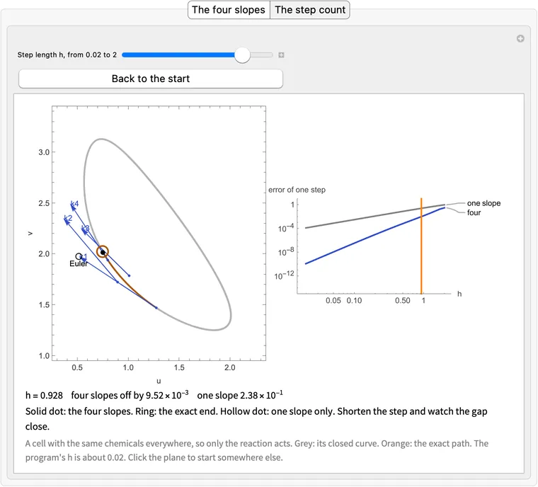
      

      Download ff-slide.wl

      A map of every shift of the waited frame against q, one cell black at T/3, beside the ringed shift's black difference, over the best any shift can do against the wait.
      What this draws, in Wolfram 15.0, 00:03
      lag = slide(third) - q                      # zero on the film

      What: third, slid back, minus q. On the film they are the same picture, so this field is zero; off it, whatever is left is the lag.

      Why: it is one field that holds everything still wrong with q and T. The next lines read their answers from it: when to stop, and how far is off.

      Try it: put off by a little, then look inside a real run

      q

      slide(third)

      lag, black is zero

      the part along

      rms(lag) with speed

      On the film, the lag is exactly the timing error

      Write for a frame of the film, for its true period, for simulate over , for slide and for rate, the speed. The rule is . Now let . Since commutes with ,

      So the lag is the speed field times , and rms(lag) is rms(speed), with rms(speed) 0.5717 at this frame. At the formula gives , measured , cosine with speed 0.99999998. Even at the cosine is 0.9983 (find-film-modes.json, block m4_T_step). The demo computes these live, for from up.

      In a run the lag is mostly not timing

      Near the film, with , and the derivative of at , the lag is . So a piece of along a mode of with factor shows up multiplied by .

      That says what the lag can see and what it cannot.

      • The time shift has : invisible. Moving along the loop changes nothing the lag can see, as it should: every place on the loop is the film. The two translations are nearly the same, and the turn line has already removed them.
      • The slow mode has : under-read. The lag shows of it, so the true distance to the film is about times the lag. Seed 1, late in the run: 4.96 times (find-film-extra-groupc.json).

      The late lag is the slow mode: from sweep to sweep it keeps its shape, cosine at least 0.987 with the sweep before, and shrinks . On seed 1 its cosine with speed goes from at sweep 15 to at the end, as the readout shows (find-film-extra-fix4.json). That number depends on where the run lands: from sweep 15 on, over seeds 5001-5400, its size runs from 0.005 to 0.593 with median 0.36 (block m4b_cos_by_phase has the curve). So the program's comment, T is off by 3 x lag / speed, holds exactly only for the first control on this card. The card on the 3 takes that up.

      "Zero on the film" goes one way: where else the lag is zero

      The lag being zero says the frame obeys the rule at this . It does not say the frame is the film. It is also zero:

      • on the rest state, at any : 0.0 at three values of , since nothing moves. A tiny field therefore has a tiny lag, which is the stop test's false positive;
      • on the film turned by , at : . Starts from of 10 to 13 land there, 10 of 10 checked;
      • on any field that slide leaves alone and that repeats after , such as a uniform field on the reaction's own cycle at three times its period.

      So the program's other lines have to keep it off those: the noise and the it starts from, and the last card of this part says what happens when they do not.

      Mathematica
      (* lag = slide(third) - q: on the film with T off by a little it is a copy of the speed field; inside a real run it is mostly not. Runs the program once and records it. About 2 s on an M5. *)
      n = 36; box = 40.;   (* a triangular mesh of n x n nodes, in a repeating box of this side *)
      a = 1.; b = 2.3;     (* the Brusselator's constants; both chemicals diffuse at rate 1 *)
      dt = 0.02;           (* the longest time step *)
      
      (* How fast the chemicals q = {u, v} are changing: diffusion plus reaction. *)
      laplacian[f_] := 2/(3 (box/n)^2) ListCorrelate[{{1, 1, 0}, {1, -6, 1}, {0, 1, 1}}, f, {2, 2}];
      rate[{u_, v_}] := {laplacian[u] + a - (b + 1) u + u^2 v, laplacian[v] + b u - u^2 v};
      
      (* Run time forward by t (fourth-order Runge-Kutta). *)
      simulate[q0_, t_] := Module[{q = q0, steps = Ceiling[t/dt], h, k1, k2, k3, k4},
         h = t/steps;
         Do[
          k1 = rate[q];
          k2 = rate[q + h/2 k1];
          k3 = rate[q + h/2 k2];
          k4 = rate[q + h k3];
          q += h/6 (k1 + 2 k2 + 2 k3 + k4),
          {steps}];
         q];
      
      (* Slide the picture by a third of the box. On the film this costs T/3 of time. *)
      slide[q_] := RotateLeft[q, {0, n/3, 2 n/3}];
      
      (* Turn the picture 120 degrees about the origin. On the film this costs no time. *)
      turn[q_] := Table[f[[Mod[x - y, n] + 1, Mod[-y, n] + 1]], {f, q}, {y, 0, n - 1}, {x, 0, n - 1}];
      
      (* Start from the rest state plus white noise, and find the film. *)
      rest = {ConstantArray[a, {n, n}], ConstantArray[b/a, {n, n}]};
      noise[s_, amp_ : 0.1] := (SeedRandom[s]; rest + RandomVariate[NormalDistribution[0, amp], {2, n, n}]);
      
      (* One run, with every sweep recorded: findFilm's lines, plus the record. *)
      lagRun[q0_] := Module[{q, T = 6.355, third, twoThirds, lag, speed, rows = {}},
         q = (q0 + turn[q0] + turn[turn[q0]])/3;
         Do[
          q = simulate[q, T];
          third = simulate[q, T/3];
          twoThirds = simulate[third, T/3];
          lag = slide[third] - q;
          AppendTo[rows, <|"q" -> q, "slid" -> slide[third], "lag" -> lag|>];
          If[RootMeanSquare[Flatten[lag]] < 1*^-10, Break[]];
          speed = rate[q];
          T -= Clip[3 Total[lag speed, 3]/Total[speed speed, 3], {-0.1, 0.1}];
          q = (q + slide[third] + slide[slide[twoThirds]])/3,
          {399}];
         {rows, T}];
      {lagRows, lagT} = lagRun[noise[1]];
      lagQ = lagRows[[-1, "q"]];          (* a frame of the film, to the program's own tolerance *)
      lagRange = MinMax[lagQ[[1]]];
      
      (* The cosine of two fields, each as one long list of numbers. *)
      lagCos[f_, g_] := Total[f g, 3]/Sqrt[Total[f f, 3] Total[g g, 3]];
      
      (* |u| of a difference on the plane: black is zero, white is hi. *)
      lagGrey[u_, hi_] := Quiet[
         ImageTransformation[Image[Clip[Abs[Reverse[meshFine[u]]]/hi, {0, 1}]],
          {#[[1]] + #[[2]]/Sqrt[3.], 2 #[[2]]/Sqrt[3.]}/box + 0.5/(4 n) &, {240, 240},
          DataRange -> {{0, 1}, {0, 1}}, PlotRange -> {{-40., 40.}, {-40., 40.}},
          Padding -> "Periodic", Resampling -> "Linear"],
         RemoveAlphaChannel::imginv];
      
      (* Four points a mesh step, linear on the mesh's own triangles, as the page paints: a turned field then draws as the turned picture. *)
      meshTent = Table[Max[0., 1. - Max[Abs[i], Abs[j], Abs[i - j]]/4.], {j, -3, 3}, {i, -3, 3}];
      meshFine[f_] := ListCorrelate[meshTent, KroneckerProduct[f, Normal[SparseArray[{{1, 1} -> 1.}, {4, 4}]]], {4, 4}];
      
      (* A field on the plane, as a picture: the mesh's two axes are 120 degrees apart. Blue is lo, white is hi. *)
      picture[u_, {lo_, hi_}, size_ : 240] := Colorize[
         Quiet[    (* Wolfram 15's ImageTransformation trips on the notebook's light/dark background, harmlessly *)
          ImageTransformation[Image[Rescale[Reverse[meshFine[u]], {lo, hi}]],
           {#[[1]] + #[[2]]/Sqrt[3.], 2 #[[2]]/Sqrt[3.]}/box + 0.5/(4 n) &, {size, size},
           DataRange -> {{0, 1}, {0, 1}}, PlotRange -> {{-40., 40.}, {-40., 40.}},
           Padding -> "Periodic", Resampling -> "Linear"],
          RemoveAlphaChannel::imginv],
         ColorFunction -> (Blend[{RGBColor[0.118, 0.165, 0.51], RGBColor[0.251, 0.329, 0.808], RGBColor[0.588, 0.667, 0.941], RGBColor[0.961, 0.973, 1.]}, #] &), ColorFunctionScaling -> False];
      
      (* The four panes. The last is the multiple of speed closest to the lag, on the lag's scale. *)
      lagPanes[q_, slid_, lag_, speed_, hi_] := Grid[{
          Style[#, "Text", 12] & /@ {"q", "slide(third)", "lag, black is zero", "the part along speed = rate[q]"},
          Show[#, ImageSize -> 195] & /@ {picture[q[[1]], lagRange, 480], picture[slid[[1]], lagRange, 480], lagGrey[lag[[1]], hi],
            lagGrey[(speed Total[lag speed, 3]/Total[speed speed, 3])[[1]], hi]}},
         Spacings -> {0.3, 0.3}];
      
      lagFilmView[delta_] := Module[{slid = slide[simulate[lagQ, (lagT + delta)/3]], lag, speed = rate[lagQ], e},
         lag = slid - lagQ;
         e = RootMeanSquare[Flatten[lag]];
         Column[{
           lagPanes[lagQ, slid, lag, speed, 0.08],
           Style[Row[{"rms(lag) = ", ScientificForm[e, 3], "   |delta|/3 x rms(speed) = ", ScientificForm[Abs[delta]/3 RootMeanSquare[Flatten[speed]], 3],
              "   cosine with speed = ", If[e < 1*^-9, "none: no lag", NumberForm[lagCos[lag, speed], {5, 4}]]}], "Text", 13],
           Pane[TextCell[If[delta == 0, "All black: at the true T this frame obeys the rule.", "The lag is the speed field, scaled: the only thing wrong here is the timing, and the lag says so."], "Text", FontSize -> 13], 790],
           Pane[TextCell["The frame the program returned, T off by delta. White: 0.08 in u.", "Text", FontSize -> 12, FontColor -> Gray], 790]}]];
      
      lagRunView[s_] := Module[{row = lagRows[[s]], speed = rate[lagRows[[s, "q"]]], e},
         e = RootMeanSquare[Flatten[row["lag"]]];
         Column[{
           lagPanes[row["q"], row["slid"], row["lag"], speed, Max[Abs[row["lag"][[1]]]]],
           Style[Row[{"rms(lag) = ", ScientificForm[e, 3], "   cosine with speed = ", NumberForm[lagCos[row["lag"], speed], {4, 3}],
              "   cosine with last sweep's lag = ", If[s > 1, NumberForm[lagCos[row["lag"], lagRows[[s - 1, "lag"]]], {4, 3}], "none yet"]}], "Text", 13],
           Pane[TextCell[If[s < 7, "The field is still growing, and T is off: the lag is big, and only part of it is timing.",
              "Most of this lag is not along speed, so it is not timing. It is what the sweeps have yet to remove, and it keeps its shape from sweep to sweep."], "Text", FontSize -> 13], 790],
           Style[Row[{"Seed 1, sweep ", s, " of ", Length[lagRows], ". White in the two lag panes: ", ScientificForm[Max[Abs[row["lag"][[1]]]], 2], " in u, rescaled for each sweep."}], "Text", 12, Gray]}]];
      
      TabView[{
        "On the film" -> Manipulate[lagFilmView[delta], {{delta, 0.1, "T off by delta"}, -0.3, 0.3, 0.01, Appearance -> "Labeled"}, SaveDefinitions -> True],
        "In a real run" -> Manipulate[lagRunView[s], {{s, 12, "Sweep"}, 1, Length[lagRows], 1, Appearance -> "Labeled"}, SaveDefinitions -> True]}]
      

      Download ff-lag.wl

      Four panes in a row, q, the slid third, the lag and its part along speed, the last two alike when T is off by a little, with a slider on the error in T and a second tab inside a real run.
      What this draws, in Wolfram 15.0, 00:02
      if np.sqrt(np.mean(lag * lag)) < tol:
      def find_film(q, T=6.355, tol=1e-10):

      What: the of the lag, one number. Under tol, the program returns.

      Why: the lag never reaches zero, so "zero" has to mean something. is small enough that has settled to nine decimals, and big enough to be reached: this program's lag stops falling a little below it.

      Try it: move tol, and see what the run would return

      q at the stop

      its distance from the film, black is none

      stops distance to the film

      over 400 seeds

      What each tol buys, over 400 seeds

      Seeds 11001-11400, one run each, with every stop recorded on the way (find-film-runs.json, block page.tol). Medians; is the true period, and the distance is rms to the nearest frame of the exact film.

      tolstopat sweepdistance
      4007
      40011
      40015
      40021
      40026
      37029
      0raises

      Each factor of 10 costs sweeps, the slow mode's rate (the sweep's factor). The distance runs about 3 times tol from down, so the test reads the true distance fairly here.

      At the median hides two populations: 148 of 400 stop at sweep 2 or 3, on a field that has not grown, up to 0.38 from the film; the others at sweeps 6 to 10, at 0.014. Seed 1 is one of the others, by a hair: its lag at sweep 2 is 0.0116. It grows again as the pattern grows, which is why rms(lag) rises in the first sweeps of the chart.

      The floor is the time step, not round-off

      As written, rms(lag) stops falling at on seed 1, and at to over 400 seeds. Round-off is about . The cause is one line of simulate, steps = int(np.ceil(t / dt)): at a free period takes 320 steps, and three thirds take 321. Two different step sizes make two slightly different maps, so the frame the free period leaves is not quite on the film of the third's map. The kick is a period, on the exact frame.

      The experiment that could have shown otherwise: change nothing but the step count.

      steps: free, three thirdsfloor
      0.020000320, 321
      0.019920321, 321
      0.020500312, 312
      0.010000640, 642
      0.040000160, 162

      A coarser step with equal counts floors at round-off, and a finer one with unequal counts does not. The chip Free period as three thirds gives every step one length: the floor goes, and seed 1's lag falls to , with on the exact value to the last digit (find-film-extra-groupc.json).

      So tol sits only 4.3 to 17 times above the floor. A smaller tol stops being a matter of patience: stops on 370 of 400 seeds, and the rest raise after 399 sweeps, film in hand, because the floor depends on where on the loop the frame sits, and on their part of the loop it is higher. At other settings the same thing makes the program raise from on in a comb.

      Why rms, and when a small number is not the film

      On a fixed mesh any measure would do; each is a fixed multiple of the others near the end. Late in the run the largest entry of the lag is about 4.5 times the rms. Rms is the size that goes with the inner product the line uses, so the two lines agree on what "small" means. Against the field's own spread, std() 0.32 at that instant (0.28 to 0.44 round the film, find-film-extra-fix3.json), the program's tol is a relative .

      A false positive. tol is absolute, so a tiny field has a tiny lag without being a film: its first lag is about 0.32 of its amplitude. From noise of amplitude the program returns at sweep 1, 100 of 100, with no pattern at all. A small field goes on coming back, by sweep 2, up to amplitude (100 of 100, of which 17 at sweep 1), and that dies out by . So a caller should check std() and ; this line will not (what else it misses).

      Mathematica
      (* The stop test: rms(lag) against the sweep with tol as a line, the sweep the run would stop at, the frame it would return and how far that is from the film; and the same with the free period run as three thirds, which removes the floor. About 7 s on an M5. *)
      
      n = 36; box = 40.;   (* a triangular mesh of n x n nodes, in a repeating box of this side *)
      a = 1.; b = 2.3;     (* the Brusselator's constants; both chemicals diffuse at rate 1 *)
      dt = 0.02;           (* the longest time step *)
      
      (* How fast the chemicals q = {u, v} are changing: diffusion plus reaction. *)
      laplacian[f_] := 2/(3 (box/n)^2) ListCorrelate[{{1, 1, 0}, {1, -6, 1}, {0, 1, 1}}, f, {2, 2}];
      rate[{u_, v_}] := {laplacian[u] + a - (b + 1) u + u^2 v, laplacian[v] + b u - u^2 v};
      
      (* Run time forward by t (fourth-order Runge-Kutta). *)
      simulate[q0_, t_] := Module[{q = q0, steps = Ceiling[t/dt], h, k1, k2, k3, k4},
         h = t/steps;
         Do[
          k1 = rate[q];
          k2 = rate[q + h/2 k1];
          k3 = rate[q + h/2 k2];
          k4 = rate[q + h k3];
          q += h/6 (k1 + 2 k2 + 2 k3 + k4),
          {steps}];
         q];
      
      (* Slide the picture by a third of the box. On the film this costs T/3 of time. *)
      slide[q_] := RotateLeft[q, {0, n/3, 2 n/3}];
      
      (* Turn the picture 120 degrees about the origin. On the film this costs no time. *)
      turn[q_] := Table[f[[Mod[x - y, n] + 1, Mod[-y, n] + 1]], {f, q}, {y, 0, n - 1}, {x, 0, n - 1}];
      
      (* One frame of the film, its period T, and the number of sweeps it took. *)
      findFilm[q0_, T0_ : 6.355, tol_ : 1*^-10] := Module[{q, T = T0, third, twoThirds, lag, speed},
         q = (q0 + turn[q0] + turn[turn[q0]])/3;    (* costs no time, so impose it once and it stays *)
         Do[
          q = simulate[q, T];                       (* one free period: what decays, decays *)
          third = simulate[q, T/3];
          twoThirds = simulate[third, T/3];
      
          lag = slide[third] - q;                   (* zero on the film *)
          If[RootMeanSquare[Flatten[lag]] < tol, Return[{q, T, sweep}, Module]];
      
          (* T is off by 3 x lag / speed. Move it gently, since at first it's all noise. *)
          speed = rate[q];
          T -= Clip[3 Total[lag speed, 3]/Total[speed speed, 3], {-0.1, 0.1}];
      
          (* What obeys the rule survives the average; what ticks in unison cancels. *)
          q = (q + slide[third] + slide[slide[twoThirds]])/3,
          {sweep, 399}];
         $Failed];
      
      (* Start from the rest state plus white noise, and find the film. *)
      rest = {ConstantArray[a, {n, n}], ConstantArray[b/a, {n, n}]};
      noise[s_, amp_ : 0.1] := (SeedRandom[s]; rest + RandomVariate[NormalDistribution[0, amp], {2, n, n}]);
      
      (* Four points a mesh step, linear on the mesh's own triangles, as the page paints: a turned field then draws as the turned picture. *)
      meshTent = Table[Max[0., 1. - Max[Abs[i], Abs[j], Abs[i - j]]/4.], {j, -3, 3}, {i, -3, 3}];
      meshFine[f_] := ListCorrelate[meshTent, KroneckerProduct[f, Normal[SparseArray[{{1, 1} -> 1.}, {4, 4}]]], {4, 4}];
      
      (* A field on the plane, as a picture: the mesh's two axes are 120 degrees apart. Blue is lo, white is hi. *)
      picture[u_, {lo_, hi_}, size_ : 240] := Colorize[
         Quiet[    (* Wolfram 15's ImageTransformation trips on the notebook's light/dark background, harmlessly *)
          ImageTransformation[Image[Rescale[Reverse[meshFine[u]], {lo, hi}]],
           {#[[1]] + #[[2]]/Sqrt[3.], 2 #[[2]]/Sqrt[3.]}/box + 0.5/(4 n) &, {size, size},
           DataRange -> {{0, 1}, {0, 1}}, PlotRange -> {{-40., 40.}, {-40., 40.}},
           Padding -> "Periodic", Resampling -> "Linear"],
          RemoveAlphaChannel::imginv],
         ColorFunction -> (Blend[{RGBColor[0.118, 0.165, 0.51], RGBColor[0.251, 0.329, 0.808], RGBColor[0.588, 0.667, 0.941], RGBColor[0.961, 0.973, 1.]}, #] &), ColorFunctionScaling -> False];
      
      (* findFilm's loop, run on past the stop, keeping every sweep. With thirds, the free period is three thirds, so every step has one length. *)
      stopRun[q0_, thirds_] := Module[{q = (q0 + turn[q0] + turn[turn[q0]])/3, T = 6.355, third, twoThirds, lag, speed, row},
         Table[
          q = If[thirds, Nest[simulate[#, T/3] &, q, 3], simulate[q, T]];
          third = simulate[q, T/3];
          twoThirds = simulate[third, T/3];
          lag = slide[third] - q;
          row = <|"q" -> q, "T" -> T, "rms" -> RootMeanSquare[Flatten[lag]]|>;
          speed = rate[q];
          T -= Clip[3 Total[lag speed, 3]/Total[speed speed, 3], {-0.1, 0.1}];
          q = (q + slide[third] + slide[slide[twoThirds]])/3;
          row,
          45]];
      stopRuns = <|"As written" -> stopRun[noise[1], False], "Free period as three thirds" -> stopRun[noise[1], True]|>;
      
      (* The film, for measuring against: the three-thirds run's last frame and T, every step of one length, T*/321. Its other two thirds are slides of the first. *)
      {stopExact, stopTstar} = Last[stopRuns["Free period as three thirds"]] /@ {"q", "T"};
      stopH = stopTstar/321;
      stopFilm = With[{f = NestList[simulate[#, stopH] &, stopExact, 106]}, Join[f, slide[slide[#]] & /@ f, slide /@ f]];
      
      (* A frame minus the nearest frame of the film: start from the frame before the nearest, since simulate only runs forward, then Newton on the time. *)
      stopRms[f_] := RootMeanSquare[Flatten[f]];
      stopOff[q_] := Module[{i = First[Ordering[stopRms[q - #] & /@ stopFilm, 1]], from, t = stopH, f, speed},
         from = stopFilm[[Mod[i - 2, 321] + 1]];
         Do[
          f = simulate[from, t];
          speed = rate[f];
          t = Clip[t + Total[(q - f) speed, 3]/Total[speed speed, 3], {0.001, 2 stopH}],
          {3}];
         q - simulate[from, t]];
      stopDist = Map[stopRms[stopOff[#["q"]]] &, stopRuns, {2}];
      
      (* Which sweep a tol stops at, as findFilm's own test would: 0 if never. *)
      stopAt[way_, tol_] := First[FirstPosition[#["rms"] & /@ stopRuns[way], r_ /; r < tol, {0}, {1}]];
      
      (* Measured in Python over 400 seeds, numpy's seeds 11001 to 11400: how many stop at each tol, and the median sweep. A block cannot sensibly recompute these. *)
      stopTable = <|2 -> "400 of 400 stop, median sweep 7", 3 -> "400 of 400 stop, median sweep 9", 4 -> "400 of 400 stop, median sweep 11",
         5 -> "400 of 400 stop, median sweep 13", 6 -> "400 of 400 stop, median sweep 15", 7 -> "400 of 400 stop, median sweep 18",
         8 -> "400 of 400 stop, median sweep 21", 9 -> "400 of 400 stop, median sweep 24", 10 -> "400 of 400 stop, median sweep 26",
         11 -> "370 of 400 stop, median sweep 29", 12 -> "0 of 400 stop"|>;
      stopFloor = {5.81*^-12, 2.33*^-11};   (* the floor of rms(lag) as written over those seeds: smallest and largest *)
      
      (* A field's size at each node, both chemicals, as a picture: black is zero, white is hi. The same map as picture. *)
      stopGrey[{u_, v_}, hi_] := Quiet[
         ImageTransformation[Image[Clip[Reverse[Sqrt[meshFine[u]^2 + meshFine[v]^2]]/hi, {0., 1.}]],
          {#[[1]] + #[[2]]/Sqrt[3.], 2 #[[2]]/Sqrt[3.]}/box + 0.5/(4 n) &, {240, 240},
          DataRange -> {{0, 1}, {0, 1}}, PlotRange -> {{-40., 40.}, {-40., 40.}},
          Padding -> "Periodic", Resampling -> "Linear"],
         RemoveAlphaChannel::imginv];
      
      stopChart[way_, tol_, s_] := With[{other = First[DeleteCases[Keys[stopRuns], way]]},
         ListLogPlot[{#["rms"] & /@ stopRuns[other], #["rms"] & /@ stopRuns[way]},
          Joined -> {True, True}, PlotMarkers -> {None, Automatic}, PlotStyle -> {GrayLevel[0.7], RGBColor[0.2, 0.3, 0.8]},
          PlotRange -> {{1, 45}, {1*^-16, 1}}, Frame -> True, FrameLabel -> {"sweep", "rms(lag), seed 1"}, ImageSize -> 640, AspectRatio -> 0.3,
          Epilog -> {
            {RGBColor[0.75, 0.35, 0.], Dashed, Line[{{0, Log[tol]}, {46, Log[tol]}}], Text["tol", {44, Log[tol]}, {0, -1}]},
            If[way === "As written", {Gray, Dashed, Line[{{0, Log[#]}, {46, Log[#]}}] & /@ stopFloor, Text["the floor, over 400 seeds", {6, Log[First[stopFloor]]}, {0, 1.4}]}, {}],
            If[s > 0, {RGBColor[0.75, 0.35, 0.], Line[{{s, Log[1*^-16]}, {s, 0}}]}, {}]}]];
      
      Manipulate[
       With[{tol = 10.^-e, s = stopAt[way, 10.^-e], rows = stopRuns[way]},
        With[{row = rows[[If[s > 0, s, 45]]], d = If[s > 0, stopDist[way][[s]], None]},
         Column[{
           stopChart[way, tol, s],
           Grid[{{
              Labeled[Image[picture[row["q"][[1]], MinMax[stopExact[[1]]]], ImageSize -> 220], If[s > 0, "q at sweep " <> ToString[s], "q at the last sweep kept"], Top],
              Labeled[Image[stopGrey[stopOff[row["q"]], 0.4], ImageSize -> 220], "its distance from the film, black is none", Top]}}],
           Row[{"stops ", If[s > 0, "at sweep " <> ToString[s], "never"],
             "     |T - T*| ", If[s > 0, ScientificForm[Abs[row["T"] - stopTstar], 2], "none"],
             "     distance to the film ", If[s > 0, ScientificForm[d, 2], "none"]}],
           Row[{"over 400 seeds: ", If[way === "As written", Lookup[stopTable, e, If[e > 12, "0 of 400 stop, as at 1e-12", "not in the table"]], "seed 1 only, on this setting"]}],
           Which[
            s == 0, "Never: rms(lag) stays above this tol. The program runs 399 sweeps and raises, with the film already found.",
            d > 0.05, "Stops on a field that has not become a film: the test is satisfied because the field is small.",
            way === "As written", Row[{"Stops at sweep ", s, ", with T right to about ", ScientificForm[Abs[row["T"] - stopTstar], 2], "."}],
            True, Row[{"Every step now has one length, so there is no floor. Stops at sweep ", s, "."}]]
           }, Spacings -> 0.8]]],
       {{e, 10, "tol = 10^-"}, 1, 15, 1, Appearance -> "Labeled"},
       {{way, "As written", ""}, Keys[stopRuns], ControlType -> SetterBar},
       BaseStyle -> {FontFamily -> "Helvetica"}, SaveDefinitions -> True]
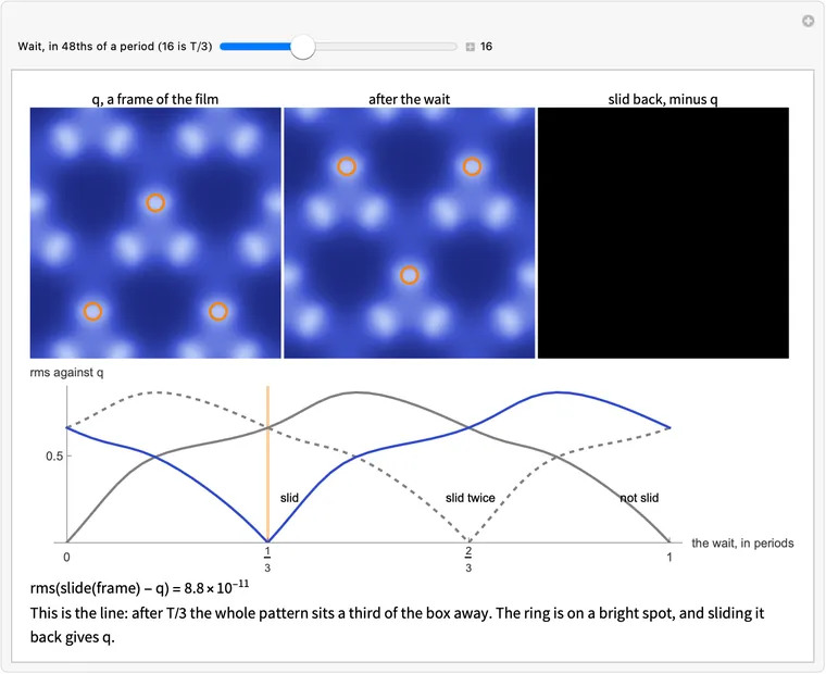
      

      Download ff-stop.wl

      rms(lag) against the sweep on a log axis with tol as a line, above the frame the run would return and its distance from the film, with sliders for tol and chips for how the free period runs.
      What this draws, in Wolfram 15.0, 00:07
      return q, T, sweep

      What: the frame that passed the test, the it was tested with, and how many it took. simulate makes every other frame from these.

      Why: the film is a closed loop, and any point on it will do: nothing on the loop is better than the rest. So different noise lands at different places, on the same loop, with the same . They do not land evenly, though: the line steers them.

      Try it: press New noise, and see where a run lands on the loop

      The film as a ; each dot one run

      The frame returned

      this run: sweeps distance to the film

      recorded runs within of a mark (, , ) if spread evenly

      A dot's angle is where the run landed. Dots at one place stack inward, so they can be counted. The orange dot is the newest run, drawn where it really is.

      Why they bunch: the line steers, and then nothing pulls back

      Once a frame is on the loop it stays very nearly where it is: the time shift is the mode with factor 1, so the sweep does not bring it back. So the place is settled earlier. 120 seeds as written, recorded to the program's own tol, and 60 from the same noise with frozen at the true (find-film-modes.json, block m6b_landings):

      within of a thirdRayleigh
      as written62.5%0.689
      frozen at 15%0.0180.98

      is the size of the average of , the place measured over a third of the period: 1 means all in one spot, 0 means evenly spread. So the program's line picks the place, not the noise. What it does: while the pattern grows, differs from the state's own clock at that amplitude, so a sweep of moves the state round by the difference. The slope over 323 sweeps is 61.4 per unit of against 56.3 expected, correlation 0.887. 69.7% of those moves go toward the loop's smaller radius, and with frozen 38.3%. The radius is least at instant modulo , about where the dots gather ( is the time along the film from the exact frame). This is a controlled experiment and a fit, not a derivation.

      The bunching changes with the settings (200 seeds each, find-film-runs.json, block landing_phase; the same , for the same place):

      setting
      as written0.65
      noise 0.81
      noise 10.14
      two free periods0.03
      clip at 0.010.34
      frozen at 0.04

      The loop itself is a rounded triangle, not a circle: radius 18.35 to 25.25 on 144 frames, with period . Being three lobes, it holds three copies of each place; that is what makes three arcs. The dots stack inward in this drawing only so they can be counted; each landed on the loop.

      Why it returns q and this , not what the next lines would make

      The test was on this q and this T, together. The lines below it would change both, so it returns before they run. They would have improved things a little, on seed 1's last sweep (find-film-extra-groupc.json, block returned_seed1):

      returnedone line later
      distance to the film, the average
      , after its step

      So the pair is not the best the program had in hand, by a factor well under 3. Nor is more of a solution than the average: any field starts some solution, and by these numbers the average sits a little nearer the film. The reason to return is only that the test was run on it.

      How good it is, over 120 seeds: in 6.3901599181 to 6.3901599190, distance to the film to , in 24 to 29 sweeps. Seed 1's frame comes back after its own to . The distance is measured to the exact film (the card on one frame and ), and New noise computes it live: to its nearest frame, then Newton on the time.

      The recorded dots are numpy's seeds 1 to 120. New noise uses this page's own generator, the same law but not numpy's draw for that seed (the listing's fold), so a live run's place belongs to the same distribution and need not match any dot.

      A return does not prove a film: check and std()

      return says the test passed, which is less than it sounds. The same line also returns, with no error, on settings far from these: a small field from tiny noise (the stop test), a nearly uniform field with near or under 0 from a that starts too small, or from no bound on the step (the clip), and a uniform field with near 19.2829 from a that starts too large. The last card has them all. At the program's own settings none of this happens: 200 of 200 and, on fresh seeds, 400 of 400 are the film.

      Mathematica
      (* The return: each run from fresh noise lands on the same closed loop with the same T, a dot on the loop. As written they bunch at three places, since the T line steers them; with T frozen at T* they spread. Runs the real program on 60 seeds, about two minutes on an M5, and New noise runs another, about 2 s. *)
      
      n = 36; box = 40.;   (* a triangular mesh of n x n nodes, in a repeating box of this side *)
      a = 1.; b = 2.3;     (* the Brusselator's constants; both chemicals diffuse at rate 1 *)
      dt = 0.02;           (* the longest time step *)
      
      (* How fast the chemicals q = {u, v} are changing: diffusion plus reaction. *)
      laplacian[f_] := 2/(3 (box/n)^2) ListCorrelate[{{1, 1, 0}, {1, -6, 1}, {0, 1, 1}}, f, {2, 2}];
      rate[{u_, v_}] := {laplacian[u] + a - (b + 1) u + u^2 v, laplacian[v] + b u - u^2 v};
      
      (* Run time forward by t (fourth-order Runge-Kutta). *)
      simulate[q0_, t_] := Module[{q = q0, steps = Ceiling[t/dt], h, k1, k2, k3, k4},
         h = t/steps;
         Do[
          k1 = rate[q];
          k2 = rate[q + h/2 k1];
          k3 = rate[q + h/2 k2];
          k4 = rate[q + h k3];
          q += h/6 (k1 + 2 k2 + 2 k3 + k4),
          {steps}];
         q];
      
      (* Slide the picture by a third of the box. On the film this costs T/3 of time. *)
      slide[q_] := RotateLeft[q, {0, n/3, 2 n/3}];
      
      (* Turn the picture 120 degrees about the origin. On the film this costs no time. *)
      turn[q_] := Table[f[[Mod[x - y, n] + 1, Mod[-y, n] + 1]], {f, q}, {y, 0, n - 1}, {x, 0, n - 1}];
      
      (* One frame of the film, its period T, and the number of sweeps it took. *)
      findFilm[q0_, T0_ : 6.355, tol_ : 1*^-10] := Module[{q, T = T0, third, twoThirds, lag, speed},
         q = (q0 + turn[q0] + turn[turn[q0]])/3;    (* costs no time, so impose it once and it stays *)
         Do[
          q = simulate[q, T];                       (* one free period: what decays, decays *)
          third = simulate[q, T/3];
          twoThirds = simulate[third, T/3];
      
          lag = slide[third] - q;                   (* zero on the film *)
          If[RootMeanSquare[Flatten[lag]] < tol, Return[{q, T, sweep}, Module]];
      
          (* T is off by 3 x lag / speed. Move it gently, since at first it's all noise. *)
          speed = rate[q];
          T -= Clip[3 Total[lag speed, 3]/Total[speed speed, 3], {-0.1, 0.1}];
      
          (* What obeys the rule survives the average; what ticks in unison cancels. *)
          q = (q + slide[third] + slide[slide[twoThirds]])/3,
          {sweep, 399}];
         $Failed];
      
      (* Start from the rest state plus white noise, and find the film. *)
      rest = {ConstantArray[a, {n, n}], ConstantArray[b/a, {n, n}]};
      noise[s_, amp_ : 0.1] := (SeedRandom[s]; rest + RandomVariate[NormalDistribution[0, amp], {2, n, n}]);
      
      (* Four points a mesh step, linear on the mesh's own triangles, as the page paints: a turned field then draws as the turned picture. *)
      meshTent = Table[Max[0., 1. - Max[Abs[i], Abs[j], Abs[i - j]]/4.], {j, -3, 3}, {i, -3, 3}];
      meshFine[f_] := ListCorrelate[meshTent, KroneckerProduct[f, Normal[SparseArray[{{1, 1} -> 1.}, {4, 4}]]], {4, 4}];
      
      (* A field on the plane, as a picture: the mesh's two axes are 120 degrees apart. Blue is lo, white is hi. *)
      picture[u_, {lo_, hi_}, size_ : 240] := Colorize[
         Quiet[    (* Wolfram 15's ImageTransformation trips on the notebook's light/dark background, harmlessly *)
          ImageTransformation[Image[Rescale[Reverse[meshFine[u]], {lo, hi}]],
           {#[[1]] + #[[2]]/Sqrt[3.], 2 #[[2]]/Sqrt[3.]}/box + 0.5/(4 n) &, {size, size},
           DataRange -> {{0, 1}, {0, 1}}, PlotRange -> {{-40., 40.}, {-40., 40.}},
           Padding -> "Periodic", Resampling -> "Linear"],
          RemoveAlphaChannel::imginv],
         ColorFunction -> (Blend[{RGBColor[0.118, 0.165, 0.51], RGBColor[0.251, 0.329, 0.808], RGBColor[0.588, 0.667, 0.941], RGBColor[0.961, 0.973, 1.]}, #] &), ColorFunctionScaling -> False];
      
      {retFrame, retT, retSweeps} = findFilm[noise[1]];
      
      (* The film, to measure against: the same sweep with every step of one length (T/321) goes on down past the floor, so 20 more sweeps polish the frame. *)
      retPolish[{q_, T_}] := Module[{free = Nest[simulate[#, T/3] &, q, 3], third, twoThirds, lag, speed},
         third = simulate[free, T/3];
         twoThirds = simulate[third, T/3];
         lag = slide[third] - free;
         speed = rate[free];
         {(free + slide[third] + slide[slide[twoThirds]])/3, T - 3 Total[lag speed, 3]/Total[speed speed, 3]}];
      {retExact, retTstar} = Nest[retPolish, {retFrame, retT}, 20];
      retH = retTstar/321;
      retFilm = With[{f = NestList[simulate[#, retH] &, retExact, 106]}, Join[f, slide[slide[#]] & /@ f, slide /@ f]];
      
      (* The plane of the loop: the film's two main directions. The marks 0, T/3, 2T/3 are where the loop's radius is least, and place 0 is the first of them. *)
      retCentre = Mean[Flatten /@ retFilm];
      retAxes = Transpose[Last[SingularValueDecomposition[(# - retCentre &) /@ (Flatten /@ retFilm[[;; ;; 4]]), 2]]];
      retXY[q_] := retAxes . (Flatten[q] - retCentre);
      retLoop = retXY /@ retFilm;
      retZero = First[Ordering[Norm /@ retLoop, 1]];
      
      (* findFilm's loop as written, or with T held frozen at T*, keeping where q walks in the plane. *)
      retRun[s_, frozen_] := Module[{q = noise[s], T = If[frozen, retTstar, 6.355], third, twoThirds, lag, speed, trail = {}, done = False, sweeps = 0},
         q = (q + turn[q] + turn[turn[q]])/3;
         While[! done && sweeps < 399,
          sweeps++;
          q = simulate[q, T];
          AppendTo[trail, retXY[q]];
          third = simulate[q, T/3];
          twoThirds = simulate[third, T/3];
          lag = slide[third] - q;
          If[RootMeanSquare[Flatten[lag]] < 1*^-10, done = True,
           speed = rate[q];
           If[! frozen, T -= Clip[3 Total[lag speed, 3]/Total[speed speed, 3], {-0.1, 0.1}]];
           q = (q + slide[third] + slide[slide[twoThirds]])/3]];
         <|"seed" -> s, "q" -> q, "T" -> T, "sweeps" -> sweeps, "trail" -> trail|>];
      
      (* A frame's place on the loop, a fraction of the period from mark 0, and its distance from the film: from the frame before the nearest, since simulate only runs forward, then Newton on the time. *)
      retRms[f_] := RootMeanSquare[Flatten[f]];
      retWhere[q_] := Module[{i = First[Ordering[retRms[q - #] & /@ retFilm, 1]], from, t = retH, f, speed},
         from = retFilm[[Mod[i - 2, 321] + 1]];
         Do[
          f = simulate[from, t];
          speed = rate[f];
          t = Clip[t + Total[(q - f) speed, 3]/Total[speed speed, 3], {0.001, 2 retH}],
          {3}];
         <|"place" -> Mod[(i - 2 - retZero + 1)/321. + t/retTstar, 1], "dist" -> retRms[q - simulate[from, t]]|>];
      
      retNew[way_, s_] := With[{r = retRun[s, way =!= "As written"]}, Join[r, retWhere[r["q"]]]];
      retRuns = <|"As written" -> Table[retNew["As written", s], {s, 20}], "T frozen at T*" -> Table[retNew["T frozen at T*", s], {s, 40}]|>;
      
      (* The share within T/36 of a mark. *)
      retShare[runs_] := N[Count[runs, r_ /; With[{m = Mod[r["place"], 1/3]}, Min[m, 1/3 - m] <= 1/36]]/Length[runs]];
      (* Measured in Python, numpy's seeds, each to tol 1e-10, about the same marks: *)
      retRecorded = <|"As written" -> "62.5% of 120, bunching R = 0.69", "T frozen at T*" -> "15.0% of 60, bunching R = 0.02"|>;
      
      (* Dots on the loop: a dot's angle is where the run landed, and dots at one place stack inward so that they can be counted. *)
      retDots[runs_] := Module[{count = <||>, b},
         Table[
          b = Floor[36 r["place"]];
          count[b] = Lookup[count, b, -1] + 1;
          (1 - 0.04 count[b]) retLoop[[Mod[retZero + Round[(b + 0.5)/36 321] - 1, 321] + 1]],
          {r, runs}]];
      
      retPicture[runs_] := With[{now = Last[runs]},
         Graphics[{
           {GrayLevel[0.65], Thick, Line[Append[retLoop, First[retLoop]]]},
           {Gray, Text["+", {0, 0}]},
           MapThread[{Gray, Text[#1, 1.18 retLoop[[Mod[retZero + #2 - 1, 321] + 1]]]} &, {{"0", "T/3", "2T/3"}, {0, 107, 214}}],
           {RGBColor[0.2, 0.3, 0.8], PointSize[0.014], Point[retDots[runs]]},
           {RGBColor[0.2, 0.3, 0.8], Line[now["trail"]]},
           {RGBColor[0.75, 0.35, 0.], PointSize[0.03], Point[retXY[now["q"]]]}},
          ImageSize -> 360, PlotRange -> 31]];
      
      Manipulate[
       With[{runs = retRuns[way]},
        With[{now = Last[runs]},
         Column[{
           Grid[{{
              Labeled[retPicture[runs], "The film as a loop; each dot one run", Top],
              Labeled[Image[picture[now["q"][[1]], MinMax[retExact[[1]]]], ImageSize -> 260], "The frame returned, orange dot", Top]}}],
           Row[{"this run: seed ", now["seed"], "     sweeps ", now["sweeps"], "     T ", NumberForm[now["T"], 11], "     distance to the film ", ScientificForm[now["dist"], 2]}],
           Row[{"runs within T/36 of a mark ", PercentForm[retShare[runs], 3], " of ", Length[runs], "     if spread evenly 16.7%     recorded in Python: ", retRecorded[way]}],
           If[way === "As written",
            "Same loop, same T, and they gather at the same places. The T line steers runs there.",
            "With T frozen at T* the runs spread round the loop: the bunching was the T line's doing."]
           }, Spacings -> 0.8]]],
       {{way, "As written", ""}, Keys[retRuns], ControlType -> SetterBar},
       {{pressed, 0}, ControlType -> None},
       Button["New noise",
        With[{s = Max[#["seed"] & /@ retRuns[way]] + 1}, AppendTo[retRuns[way], retNew[way, s]]]; pressed++, Method -> "Queued"],
       TrackedSymbols :> {way, pressed},
       BaseStyle -> {FontFamily -> "Helvetica"}, SaveDefinitions -> True]
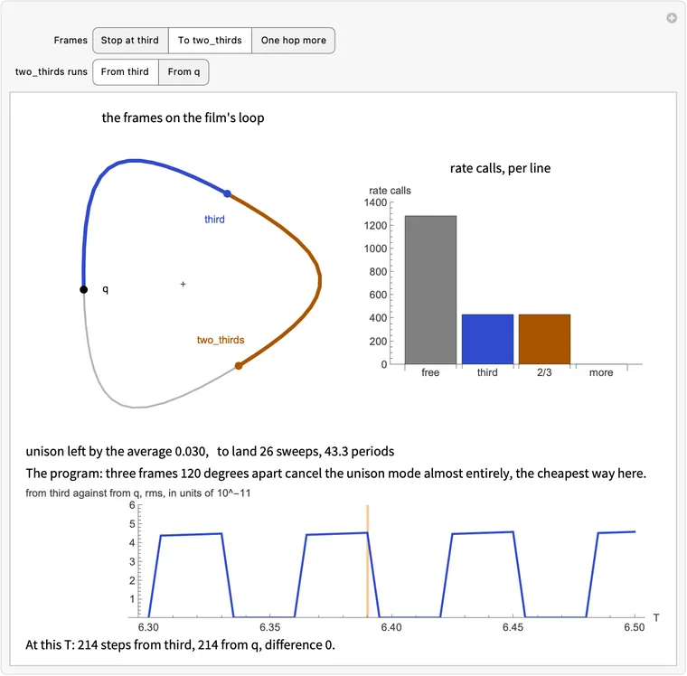
      

      Download ff-return.wl

      The film's closed loop with one dot per run from fresh noise, bunched at three places, an orange newest run with its trail from the rest state, beside the frame it returned, with a New noise button.
      What this draws, in Wolfram 15.0, 02:08
      frame, T, sweeps = find_film(rest + 0.1 * noise)

      What: the returned frame cannot be played for ever by simulating it. Keep running simulate from it, and the film lasts about 173 periods, then dissolves into a field that moves in unison.

      Why: the film is unstable: one of it grows a period. So a player loops stored frames, and the program cannot be just a long simulation: the average is what holds the film there.

      Try it: keep simulating the returned frame, period by period

      The frame returned

      Simulated on

      distance to the film spread std()

      What grows, and at what rate

      The chart is recorded: numpy seed 1, the distance every 5 periods, a stored picture at each stop of the slider.

      The unison mode has : a disturbance of that shape, placed on the exact frame by hand, grows by a period (find-film-modes.json, block m10_unison). The name is loose: about 60.7% of the mode is a change in the spatial mean, and the rest is not.

      In the chart the distance grows more slowly, about a period. Both are right: the deviation turns a period in the plane of that complex mode, on which its rms is not constant. Rebuilt from the mode's amplitude, that gives , against measured (find-film-runs.json, block after_return).

      First the distance falls, from to by period 10: the slow mode, which tol left in the frame, decays on its own (read from the rate, not projected on the mode). Only what lies on the growing mode remains.

      At the end the field is nearly uniform, spread under , with period 6.4276: the reaction's own cycle, the third of three clocks, after the rest state's and the film's 6.3902 (the card on the guess). The dates, over seeds 17001-17040: the distance passes a tenth of the spread at period 155 to 158, the spread halves at 167 to 179, and it falls under 1% at 188 to 199.

      What sets the date: not tol, but 320 steps against 321

      A guess would be that a frame good to has that much of the growing mode in it. It has about , read from the date itself. And a better frame does not last longer. Spread halved at:

      starthow it is runperiod
      a returned frame, seed 1simulate(q, T)172
      the exact frame, lag simulate(q, T)174
      the exact framethree thirds, its own step length251
      the exact frame + of the modesimulate(q, T)151

      An exact frame under simulate(q, T) lasts no longer than a returned one, since 320 steps kick it by at once, against the 321 steps it was solved on: the same mismatch as the floor. Run on its own step length it goes on until round-off starts the mode, and that is a draw: 224 to 257 periods to a tenth of the spread. At , each extra decade of precision buys about 15 periods, so no precision helps much.

      Why the program is not a long simulation, and how a player plays it

      Simulation alone cannot find the film. From noise, with the average removed and frozen even at the true value, the field ends in unison, 20 of 20 (find-film-runs.json). This card is the same fact seen from the far end: the film is not where free running goes.

      What makes the sweep different is one number. A sweep's free period multiplies that mode by 1.16, and the average then multiplies it by 0.0303: 0.0351 in all, measured 0.0351. So the sweep has a stable film where the free run has an unstable one (the filter). Only the factor changes, not the film: the map's fixed point is an exact solution of the equation.

      A player therefore does not simulate. It stores one period's frames and loops them, as the demo in section 16 does, which is why the returned matters as much as the frame: it says how long the loop must be.

      Mathematica
      (* What the returned frame cannot do: keep simulating it, and the distance from the film falls, then grows in a straight line on a log axis until the pattern dissolves into a field that moves in unison. About 16 s on an M5. *)
      
      n = 36; box = 40.;   (* a triangular mesh of n x n nodes, in a repeating box of this side *)
      a = 1.; b = 2.3;     (* the Brusselator's constants; both chemicals diffuse at rate 1 *)
      dt = 0.02;           (* the longest time step *)
      
      (* How fast the chemicals q = {u, v} are changing: diffusion plus reaction. *)
      laplacian[f_] := 2/(3 (box/n)^2) ListCorrelate[{{1, 1, 0}, {1, -6, 1}, {0, 1, 1}}, f, {2, 2}];
      rate[{u_, v_}] := {laplacian[u] + a - (b + 1) u + u^2 v, laplacian[v] + b u - u^2 v};
      
      (* Run time forward by t (fourth-order Runge-Kutta). *)
      simulate[q0_, t_] := Module[{q = q0, steps = Ceiling[t/dt], h, k1, k2, k3, k4},
         h = t/steps;
         Do[
          k1 = rate[q];
          k2 = rate[q + h/2 k1];
          k3 = rate[q + h/2 k2];
          k4 = rate[q + h k3];
          q += h/6 (k1 + 2 k2 + 2 k3 + k4),
          {steps}];
         q];
      
      (* Slide the picture by a third of the box. On the film this costs T/3 of time. *)
      slide[q_] := RotateLeft[q, {0, n/3, 2 n/3}];
      
      (* Turn the picture 120 degrees about the origin. On the film this costs no time. *)
      turn[q_] := Table[f[[Mod[x - y, n] + 1, Mod[-y, n] + 1]], {f, q}, {y, 0, n - 1}, {x, 0, n - 1}];
      
      (* One frame of the film, its period T, and the number of sweeps it took. *)
      findFilm[q0_, T0_ : 6.355, tol_ : 1*^-10] := Module[{q, T = T0, third, twoThirds, lag, speed},
         q = (q0 + turn[q0] + turn[turn[q0]])/3;    (* costs no time, so impose it once and it stays *)
         Do[
          q = simulate[q, T];                       (* one free period: what decays, decays *)
          third = simulate[q, T/3];
          twoThirds = simulate[third, T/3];
      
          lag = slide[third] - q;                   (* zero on the film *)
          If[RootMeanSquare[Flatten[lag]] < tol, Return[{q, T, sweep}, Module]];
      
          (* T is off by 3 x lag / speed. Move it gently, since at first it's all noise. *)
          speed = rate[q];
          T -= Clip[3 Total[lag speed, 3]/Total[speed speed, 3], {-0.1, 0.1}];
      
          (* What obeys the rule survives the average; what ticks in unison cancels. *)
          q = (q + slide[third] + slide[slide[twoThirds]])/3,
          {sweep, 399}];
         $Failed];
      
      (* Start from the rest state plus white noise, and find the film. *)
      rest = {ConstantArray[a, {n, n}], ConstantArray[b/a, {n, n}]};
      noise[s_, amp_ : 0.1] := (SeedRandom[s]; rest + RandomVariate[NormalDistribution[0, amp], {2, n, n}]);
      
      (* Four points a mesh step, linear on the mesh's own triangles, as the page paints: a turned field then draws as the turned picture. *)
      meshTent = Table[Max[0., 1. - Max[Abs[i], Abs[j], Abs[i - j]]/4.], {j, -3, 3}, {i, -3, 3}];
      meshFine[f_] := ListCorrelate[meshTent, KroneckerProduct[f, Normal[SparseArray[{{1, 1} -> 1.}, {4, 4}]]], {4, 4}];
      
      (* A field on the plane, as a picture: the mesh's two axes are 120 degrees apart. Blue is lo, white is hi. *)
      picture[u_, {lo_, hi_}, size_ : 240] := Colorize[
         Quiet[    (* Wolfram 15's ImageTransformation trips on the notebook's light/dark background, harmlessly *)
          ImageTransformation[Image[Rescale[Reverse[meshFine[u]], {lo, hi}]],
           {#[[1]] + #[[2]]/Sqrt[3.], 2 #[[2]]/Sqrt[3.]}/box + 0.5/(4 n) &, {size, size},
           DataRange -> {{0, 1}, {0, 1}}, PlotRange -> {{-40., 40.}, {-40., 40.}},
           Padding -> "Periodic", Resampling -> "Linear"],
          RemoveAlphaChannel::imginv],
         ColorFunction -> (Blend[{RGBColor[0.118, 0.165, 0.51], RGBColor[0.251, 0.329, 0.808], RGBColor[0.588, 0.667, 0.941], RGBColor[0.961, 0.973, 1.]}, #] &), ColorFunctionScaling -> False];
      
      {unsFrame, unsT, unsSweeps} = findFilm[noise[1]];
      
      (* Keep simulating, as a player that did not store its frames would: 250 periods. *)
      unsAfter = NestList[simulate[#, unsT] &, unsFrame, 250];
      
      (* The film, to measure against: the same sweep with every step of one length (T/321) goes on down past the floor, so 20 more sweeps polish the frame. *)
      unsPolish[{q_, T_}] := Module[{free = Nest[simulate[#, T/3] &, q, 3], third, twoThirds, lag, speed},
         third = simulate[free, T/3];
         twoThirds = simulate[third, T/3];
         lag = slide[third] - free;
         speed = rate[free];
         {(free + slide[third] + slide[slide[twoThirds]])/3, T - 3 Total[lag speed, 3]/Total[speed speed, 3]}];
      {unsExact, unsTstar} = Nest[unsPolish, {unsFrame, unsT}, 20];
      unsH = unsTstar/321;
      unsFilm = With[{f = NestList[simulate[#, unsH] &, unsExact, 106]}, Join[f, slide[slide[#]] & /@ f, slide /@ f]];
      
      (* The distance to the nearest frame of the film: from the frame before the nearest, since simulate only runs forward, then Newton on the time. *)
      unsRms[f_] := RootMeanSquare[Flatten[f]];
      unsDistance[q_] := Module[{i = First[Ordering[unsRms[q - #] & /@ unsFilm, 1]], from, t = unsH, f, speed},
         from = unsFilm[[Mod[i - 2, 321] + 1]];
         Do[
          f = simulate[from, t];
          speed = rate[f];
          t = Clip[t + Total[(q - f) speed, 3]/Total[speed speed, 3], {0.001, 2 unsH}],
          {3}];
         unsRms[q - simulate[from, t]]];
      unsDist = unsDistance /@ unsAfter;
      unsSpread = StandardDeviation[Flatten[#[[1]]]] & /@ unsAfter;
      
      unsLook = MinMax[unsFrame[[1]]];
      unsHalved = First[FirstPosition[unsSpread, s_ /; s < unsSpread[[1]]/2]] - 1;    (* the period at which the spread halves *)
      unsGrowth = Exp[Last[LeastSquares[Table[{1., p}, {p, 30, 130}], Table[Log[unsDist[[p + 1]]], {p, 30, 130}]]]];    (* the straight line's factor a period *)
      
      Manipulate[
       Column[{
         ListLogPlot[{Transpose[{Range[0, 250], unsSpread}], Transpose[{Range[0, 250], unsDist}], Table[{t, unsDist[[61]] unsGrowth^(t - 60)}, {t, 15, 165}]},
          Joined -> True, PlotStyle -> {GrayLevel[0.65], RGBColor[0.2, 0.3, 0.8], Directive[RGBColor[0.75, 0.35, 0.], Dashed]},
          PlotRange -> {{0, 250}, {1*^-12, 3}}, Frame -> True, FrameLabel -> {"periods simulated", "rms, log axis"},
          ImageSize -> 620, AspectRatio -> 0.33, Epilog -> {
            {RGBColor[0.75, 0.35, 0.], Line[{{p, Log[1*^-12]}, {p, Log[3]}}]},
            {GrayLevel[0.45], Text["spread", {232, Log[unsSpread[[233]]]}, {-1.2, -0.5}]},
            {RGBColor[0.2, 0.3, 0.8], Text["distance to the film", {215, Log[unsDist[[216]]]}, {0, 1.5}]},
            {RGBColor[0.75, 0.35, 0.], Text["\[Times] " <> ToString[NumberForm[unsGrowth, 4]] <> " a period", {95, Log[unsDist[[61]] unsGrowth^35]}, {1.2, -1}]}}],
         Grid[{{
            Labeled[Image[picture[unsAfter[[1, 1]], unsLook], ImageSize -> 220], "The frame returned", Top],
            Labeled[Image[picture[unsAfter[[p + 1, 1]], unsLook], ImageSize -> 220], If[p == 0, "The same frame", "After " <> ToString[p] <> " periods"], Top]}}],
         Row[{"distance to the film ", ScientificForm[unsDist[[p + 1]], 3], "     spread std(u) ", NumberForm[unsSpread[[p + 1]], 4]}],
         Which[
          unsSpread[[p + 1]] <= 0.01 unsSpread[[1]], "The pattern has gone. What is left is nearly uniform, ticking on the reaction's own cycle.",
          unsDist[[p + 1]] > 0.5 unsSpread[[p + 1]], "The growing mode has reached the size of the pattern, and the pattern is going.",
          p == 0, "The frame the program returned.",
          True, "To the eye nothing has happened, yet the distance has grown: a straight line on this axis is a fixed factor a period."],
         Row[{"This run: the spread halved at period ", unsHalved, ". Over 40 seeds in Python (numpy seeds 17001 to 17040): 167 to 179."}]
         }, Spacings -> 0.8],
       {{p, 175, "Periods simulated"}, 0, 250, 5, Appearance -> "Labeled"},
       BaseStyle -> {FontFamily -> "Helvetica"}, SaveDefinitions -> True]
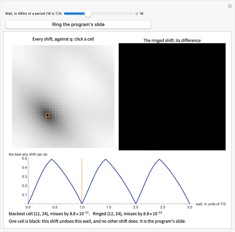
      

      Download ff-unstable.wl

      The distance from the film against periods simulated on a log axis, falling and then growing in a straight line while the spread stays flat and then drops, beside the returned frame and the same frame after the slider's periods.
      What this draws, in Wolfram 15.0, 00:16

      23. Correcting the period

      The program does not know the period. These lines read the error in from lag and take it off. On the exact film that reading is right up to a term in . In a real run one step takes off only about 0.57 of the error, and the card on the 3 shows why.

      speed = rate(q)

      What: how fast each chemical at each node is changing right now. It is one field, the same shape as q.

      Why: a frame that is a short time out of step sits speed away from where it should be. So speed is what a timing error looks like, and the next lines look for it in lag.

      Try it: shorten the time and watch the difference go black

      change over , per unit time

      speed = rate(q)

      their difference, black is zero

      on the film's loop

      rms(difference) rms(difference) rms(speed)

      Why a timing error looks like speed: the expansion and its test

      Write for simulate over a time , and for rate. is the right-hand side of the equation, so has the expansion

      with the derivative of rate with respect to the field. Two things follow. A frame reached too late differs by , to first order. And the two panes above differ by

      so their difference should fall in proportion to , with the constant 0.3816 on the first frame (find-film-extra-D.json). The second number in the readout is that constant, once is small.

      The test. On the exact frame, in Python (find-film-modes.json, block m7_speed):

      0.10.01
      rms(difference)0.03830.0038

      The slope of the logarithms from to is 1.0002. Below the difference rises again: that is round-off in , which has nothing to do with the film.

      What speed is on the film, and what it is in a run

      It is the tangent to the loop. Finite differences along the loop agree in direction with speed projected on its plane: cosine at least 0.9999 at all 48 frames (find-film-modes.json, block m7_speed). The plane is a shadow: only 73.5% to 92.7% of the speed's length lies in it, so the arrows above are shadows too.

      The film does not run at a constant rate. rms(speed) goes from 0.397 to 0.658 along it. That is why the second slider changes the third reading, and why a timing error of one size gives lags of different sizes.

      It is the neutral mode. Running first for and then for (the film's true period) is the same as the other order: . Differentiate in at a frame of the film, where , and : a nudge along neither grows nor shrinks. Measured with , the map from a frame to its slid frame a third of a period on: , the size of the time-stepping error. The card on the return uses this.

      In a run it is just rate. The line takes any field. Near the start the field is close to rest, so speed is small: rms 0.031 at sweep 1, the median of seeds 1-20, against 0.572 on the film. The clip's card shows what that does to the quotient.

      Cost. One call of rate out of about 2137 in a sweep. It comes after the stop test, so the last sweep skips it.

      Mathematica
      (* speed = rate[q]: the change over a short time, per unit time, beside rate[q] and their difference, which goes black as the time shrinks; on the film's loop, the chord turns into the tangent. About 2 s on an M5. *)
      
      n = 36; box = 40.;   (* a triangular mesh of n x n nodes, in a repeating box of this side *)
      a = 1.; b = 2.3;     (* the Brusselator's constants; both chemicals diffuse at rate 1 *)
      dt = 0.02;           (* the longest time step *)
      
      (* How fast the chemicals q = {u, v} are changing: diffusion plus reaction. *)
      laplacian[f_] := 2/(3 (box/n)^2) ListCorrelate[{{1, 1, 0}, {1, -6, 1}, {0, 1, 1}}, f, {2, 2}];
      rate[{u_, v_}] := {laplacian[u] + a - (b + 1) u + u^2 v, laplacian[v] + b u - u^2 v};
      
      (* Run time forward by t (fourth-order Runge-Kutta). *)
      simulate[q0_, t_] := Module[{q = q0, steps = Ceiling[t/dt], h, k1, k2, k3, k4},
         h = t/steps;
         Do[
          k1 = rate[q];
          k2 = rate[q + h/2 k1];
          k3 = rate[q + h/2 k2];
          k4 = rate[q + h k3];
          q += h/6 (k1 + 2 k2 + 2 k3 + k4),
          {steps}];
         q];
      
      (* Slide the picture by a third of the box. On the film this costs T/3 of time. *)
      slide[q_] := RotateLeft[q, {0, n/3, 2 n/3}];
      
      (* Turn the picture 120 degrees about the origin. On the film this costs no time. *)
      turn[q_] := Table[f[[Mod[x - y, n] + 1, Mod[-y, n] + 1]], {f, q}, {y, 0, n - 1}, {x, 0, n - 1}];
      
      (* One frame of the film, its period T, and the number of sweeps it took. *)
      findFilm[q0_, T0_ : 6.355, tol_ : 1*^-10] := Module[{q, T = T0, third, twoThirds, lag, speed},
         q = (q0 + turn[q0] + turn[turn[q0]])/3;    (* costs no time, so impose it once and it stays *)
         Do[
          q = simulate[q, T];                       (* one free period: what decays, decays *)
          third = simulate[q, T/3];
          twoThirds = simulate[third, T/3];
      
          lag = slide[third] - q;                   (* zero on the film *)
          If[RootMeanSquare[Flatten[lag]] < tol, Return[{q, T, sweep}, Module]];
      
          (* T is off by 3 x lag / speed. Move it gently, since at first it's all noise. *)
          speed = rate[q];
          T -= Clip[3 Total[lag speed, 3]/Total[speed speed, 3], {-0.1, 0.1}];
      
          (* What obeys the rule survives the average; what ticks in unison cancels. *)
          q = (q + slide[third] + slide[slide[twoThirds]])/3,
          {sweep, 399}];
         $Failed];
      
      (* Start from the rest state plus white noise, and find the film. *)
      rest = {ConstantArray[a, {n, n}], ConstantArray[b/a, {n, n}]};
      noise[s_, amp_ : 0.1] := (SeedRandom[s]; rest + RandomVariate[NormalDistribution[0, amp], {2, n, n}]);
      
      (* Four points a mesh step, linear on the mesh's own triangles, as the page paints: a turned field then draws as the turned picture. *)
      meshTent = Table[Max[0., 1. - Max[Abs[i], Abs[j], Abs[i - j]]/4.], {j, -3, 3}, {i, -3, 3}];
      meshFine[f_] := ListCorrelate[meshTent, KroneckerProduct[f, Normal[SparseArray[{{1, 1} -> 1.}, {4, 4}]]], {4, 4}];
      
      (* A field on the plane, as a picture: the mesh's two axes are 120 degrees apart. Blue is lo, white is hi. *)
      picture[u_, {lo_, hi_}, size_ : 240] := Colorize[
         Quiet[    (* Wolfram 15's ImageTransformation trips on the notebook's light/dark background, harmlessly *)
          ImageTransformation[Image[Rescale[Reverse[meshFine[u]], {lo, hi}]],
           {#[[1]] + #[[2]]/Sqrt[3.], 2 #[[2]]/Sqrt[3.]}/box + 0.5/(4 n) &, {size, size},
           DataRange -> {{0, 1}, {0, 1}}, PlotRange -> {{-40., 40.}, {-40., 40.}},
           Padding -> "Periodic", Resampling -> "Linear"],
          RemoveAlphaChannel::imginv],
         ColorFunction -> (Blend[{RGBColor[0.118, 0.165, 0.51], RGBColor[0.251, 0.329, 0.808], RGBColor[0.588, 0.667, 0.941], RGBColor[0.961, 0.973, 1.]}, #] &), ColorFunctionScaling -> False];
      
      {spdFrame, spdT, spdSweeps} = findFilm[noise[1]];
      spdFilm = NestList[simulate[#, spdT/48] &, spdFrame, 47];    (* 48 frames round the loop *)
      
      (* The loop's plane: the two main directions of those frames. *)
      spdCentre = Mean[Flatten /@ spdFilm];
      spdAxes = Transpose[Last[SingularValueDecomposition[(# - spdCentre &) /@ (Flatten /@ spdFilm), 2]]];
      spdXY[q_] := spdAxes . (Flatten[q] - spdCentre);
      spdLoop = spdXY /@ spdFilm;
      
      (* A field's size at each node as a picture: black is zero, white is hi. The same map as picture. *)
      spdGrey[u_, hi_] := Quiet[
         ImageTransformation[Image[Clip[Reverse[Abs[meshFine[u]]]/hi, {0., 1.}]],
          {#[[1]] + #[[2]]/Sqrt[3.], 2 #[[2]]/Sqrt[3.]}/box + 0.5/(4 n) &, {240, 240},
          DataRange -> {{0, 1}, {0, 1}}, PlotRange -> {{-40., 40.}, {-40., 40.}},
          Padding -> "Periodic", Resampling -> "Linear"],
         RemoveAlphaChannel::imginv];
      
      (* Frame j of the film, short time eps: the change over eps per unit time, speed, and their difference. *)
      spdParts[j_, eps_] := Module[{q = spdFilm[[j]], speed, change},
         speed = rate[q];
         change = (simulate[q, eps] - q)/eps;
         <|"q" -> q, "speed" -> speed, "change" -> change, "diff" -> change - speed|>];
      
      spdRms[f_] := RootMeanSquare[Flatten[f]];
      
      Manipulate[
       With[{p = spdParts[j, eps], at = spdLoop[[j]]},
        With[{hi = Ceiling[10 Max[Abs[p["speed"][[1]]]]]/10., e = spdRms[p["diff"]], s = spdRms[p["speed"]]},
         Column[{
           Grid[{{
             Labeled[Image[picture[p["change"][[1]], {-hi, hi}], ImageSize -> 190], "change over \[Epsilon], per unit time", Top],
             Labeled[Image[picture[p["speed"][[1]], {-hi, hi}], ImageSize -> 190], "speed = rate[q]", Top],
             Labeled[Image[spdGrey[p["diff"][[1]], 0.3], ImageSize -> 190], "their difference, black is zero", Top],
             Labeled[Graphics[{
                {GrayLevel[0.65], Thick, Line[Append[spdLoop, First[spdLoop]]]},
                {Gray, Text["+", {0, 0}]},
                {RGBColor[0.2, 0.3, 0.8], Thick, Arrow[{at, at + 0.5 spdAxes . Flatten[p["speed"]]}]},
                {RGBColor[0.75, 0.35, 0.], Arrow[{at, at + 0.5 spdAxes . Flatten[p["change"]]}]},
                {Black, PointSize[Large], Point[at]}}, ImageSize -> 190, PlotRange -> 29], "on the film's loop", Top]}}],
           Row[{"\[Epsilon] = ", eps, "     rms(difference) ", NumberForm[e, 3], "     rms(difference)/\[Epsilon] ", NumberForm[e/eps, 3], "     rms(speed) ", NumberForm[s, 3]}],
           If[e/s > 0.1, "Too long a step: the change over this time is not yet the speed.",
            If[e/s > 0.002, "Close: each tenth of the time leaves a tenth of the difference.",
             "The two panes are one field: rate[q] is the tangent, at no cost in simulation."]],
           "Left two panes: u, on one scale. White on the difference: 0.3. On the loop, blue is speed, orange the change: each arrow is how far that velocity carries the state in half a unit of time."
           }, Spacings -> 0.8]]],
       {{eps, 0.1, "A short time \[Epsilon]"}, {2, 1, 0.3, 0.1, 0.03, 0.01, 0.001, 0.0001, 0.00001}, ControlType -> Slider},
       {{j, 1, "Where on the film, frame of 48"}, 1, 48, 1},
       BaseStyle -> {FontFamily -> "Helvetica"}, SaveDefinitions -> True]
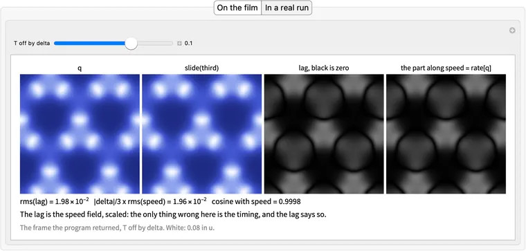
      

      Download ff-speed.wl

      The change over a time step per unit time beside rate[q] and their difference, on the blue and grey scales, and the film's loop with both as arrows, with sliders for the step and the place on the film.
      What this draws, in Wolfram 15.0, 00:02
      neighbours = [(0, 1), (0, -1), (1, 0), (-1, 0), (1, 1), (-1, -1)]
      laplacian = (sum(np.roll(q, d, (1, 2)) for d in neighbours) - 6 * q) * 2 / (3 * (L / N) ** 2)
      return laplacian + np.array([a - (b + 1) * u + u * u * v, b * u - u * u * v])

      What: the rate at a node is two things added. Diffusion pulls the node towards its six neighbours, by how far their sum sits from six times the node. The reaction is the Brusselator's law, one node at a time.

      Why: this is the equation; nowhere else does the program know any chemistry. On the film nearly all of the rate is reaction, but diffusion is what ties the nodes into one pattern, and these six neighbours treat the three directions alike, which is why the turn stays.

      Try it: tap a node, then switch the parts

      q: tap a node

      the node and its six neighbours

      In the stencil a thick spoke means the neighbour differs a lot; blue pulls the node up, orange pulls it down.

      sum of neighbours diffusion reaction rate of

      over the field: rms diffusion rms reaction

      Where comes from

      Let be the distance between neighbours, and the six vectors to them, of length and apart. Expand a smooth field about a node:

      The first sum cancels in opposite pairs. For the second, six directions apart give , since . So the sum is plus terms of order , and dividing by gives the Laplacian. That is the factor , here 0.5400, with 1.1111.

      The test. A single wave comes back multiplied by one number, within rms, and it should be near , the continuum's value (find-film-extra-D.json, block rate_parts.waves):

      on the mesh-0.0328-0.0979-0.1303-0.2894-1.0800
      -0.0329-0.0987-0.1316-0.2961-1.1844

      The film's strongest waves are the first columns, and , where the two agree to about 1%. At the top of the mesh the stencil's largest size is the factor, 4.86, which sets how long a step Runge-Kutta can take: see the card on simulate. Why takes these values on this mesh is in the card on the three waves.

      Why the turn and the slide leave it alone, and what breaks otherwise

      In the array, a turn sends a row and column offset to . The six offsets go round in two cycles of three:

      So turning the field only reorders the terms of the sum. The reaction works one node at a time, and Runge-Kutta is made of rate and sums, so simulate commutes with the turn too. Measured on the exact frame: rms . That is not quite zero only because a reordered sum can round differently. For the slide, which keeps the order, it is exactly 0 (find-film-modes.json, block m2_commute).

      The test that could fail. Swap the last two offsets for the mesh's other diagonal, : still six neighbours, the same factor, but no longer the six nearest. The commutator on the exact frame jumps to , and four neighbours give , against as written (find-film-extra-D.json, block wrong_stencil). So the symmetry is in the choice of these six and nothing else.

      How big each part is, and why the small one matters

      On the exact frame: rms diffusion 0.0305, rms reaction 0.5719, rms of the two together 0.5717. So diffusion is 5.3% of the rate there: the film is smooth, and each node is mostly a clock. On noise it is the other way round, 0.3466 against 0.2147 (seed 1, amplitude ; find-film-extra-D.json, block rate_parts).

      Small is not idle. Take the exact frame and run it for under the reaction alone, with the same Runge-Kutta. Then the slid frame misses by rms 0.0465, where the whole rate misses by (find-film-extra-D.json, block no_diffusion). Without the diffusion part this frame does not obey the rule at all, and a node's clock has nothing to keep it in step with its neighbours.

      Both chemicals use the same factor (the program's comment: "both chemicals diffuse at rate 1"). That is why every wave ticks at one frequency, the fact behind T=6.355: see the card on the guess. Each chemical's diffusion part averages to zero over the mesh, within , so it only moves chemical about.

      At rest, with , , both parts vanish: rms(rate) . So the next card's quotient, which divides by speed, is safe even there: from the exact rest state lag is already under tol, and the program returns at sweep 1, before it divides.

      Mathematica
      (* Inside rate: click a node for its six neighbours and the arithmetic of its rate; the chips show diffusion, the reaction, or both as a field, on one scale, on the film or on noise. A checkbox runs T/3 on the reaction alone, which really removes diffusion. About 2 s on an M5. *)
      
      n = 36; box = 40.;   (* a triangular mesh of n x n nodes, in a repeating box of this side *)
      a = 1.; b = 2.3;     (* the Brusselator's constants; both chemicals diffuse at rate 1 *)
      dt = 0.02;           (* the longest time step *)
      
      (* How fast the chemicals q = {u, v} are changing: diffusion plus reaction. *)
      laplacian[f_] := 2/(3 (box/n)^2) ListCorrelate[{{1, 1, 0}, {1, -6, 1}, {0, 1, 1}}, f, {2, 2}];
      rate[{u_, v_}] := {laplacian[u] + a - (b + 1) u + u^2 v, laplacian[v] + b u - u^2 v};
      
      (* Run time forward by t (fourth-order Runge-Kutta). *)
      simulate[q0_, t_] := Module[{q = q0, steps = Ceiling[t/dt], h, k1, k2, k3, k4},
         h = t/steps;
         Do[
          k1 = rate[q];
          k2 = rate[q + h/2 k1];
          k3 = rate[q + h/2 k2];
          k4 = rate[q + h k3];
          q += h/6 (k1 + 2 k2 + 2 k3 + k4),
          {steps}];
         q];
      
      (* Slide the picture by a third of the box. On the film this costs T/3 of time. *)
      slide[q_] := RotateLeft[q, {0, n/3, 2 n/3}];
      
      (* Turn the picture 120 degrees about the origin. On the film this costs no time. *)
      turn[q_] := Table[f[[Mod[x - y, n] + 1, Mod[-y, n] + 1]], {f, q}, {y, 0, n - 1}, {x, 0, n - 1}];
      
      (* One frame of the film, its period T, and the number of sweeps it took. *)
      findFilm[q0_, T0_ : 6.355, tol_ : 1*^-10] := Module[{q, T = T0, third, twoThirds, lag, speed},
         q = (q0 + turn[q0] + turn[turn[q0]])/3;    (* costs no time, so impose it once and it stays *)
         Do[
          q = simulate[q, T];                       (* one free period: what decays, decays *)
          third = simulate[q, T/3];
          twoThirds = simulate[third, T/3];
      
          lag = slide[third] - q;                   (* zero on the film *)
          If[RootMeanSquare[Flatten[lag]] < tol, Return[{q, T, sweep}, Module]];
      
          (* T is off by 3 x lag / speed. Move it gently, since at first it's all noise. *)
          speed = rate[q];
          T -= Clip[3 Total[lag speed, 3]/Total[speed speed, 3], {-0.1, 0.1}];
      
          (* What obeys the rule survives the average; what ticks in unison cancels. *)
          q = (q + slide[third] + slide[slide[twoThirds]])/3,
          {sweep, 399}];
         $Failed];
      
      (* Start from the rest state plus white noise, and find the film. *)
      rest = {ConstantArray[a, {n, n}], ConstantArray[b/a, {n, n}]};
      noise[s_, amp_ : 0.1] := (SeedRandom[s]; rest + RandomVariate[NormalDistribution[0, amp], {2, n, n}]);
      
      (* Four points a mesh step, linear on the mesh's own triangles, as the page paints: a turned field then draws as the turned picture. *)
      meshTent = Table[Max[0., 1. - Max[Abs[i], Abs[j], Abs[i - j]]/4.], {j, -3, 3}, {i, -3, 3}];
      meshFine[f_] := ListCorrelate[meshTent, KroneckerProduct[f, Normal[SparseArray[{{1, 1} -> 1.}, {4, 4}]]], {4, 4}];
      
      (* A field on the plane, as a picture: the mesh's two axes are 120 degrees apart. Blue is lo, white is hi. *)
      picture[u_, {lo_, hi_}, size_ : 240] := Colorize[
         Quiet[    (* Wolfram 15's ImageTransformation trips on the notebook's light/dark background, harmlessly *)
          ImageTransformation[Image[Rescale[Reverse[meshFine[u]], {lo, hi}]],
           {#[[1]] + #[[2]]/Sqrt[3.], 2 #[[2]]/Sqrt[3.]}/box + 0.5/(4 n) &, {size, size},
           DataRange -> {{0, 1}, {0, 1}}, PlotRange -> {{-40., 40.}, {-40., 40.}},
           Padding -> "Periodic", Resampling -> "Linear"],
          RemoveAlphaChannel::imginv],
         ColorFunction -> (Blend[{RGBColor[0.118, 0.165, 0.51], RGBColor[0.251, 0.329, 0.808], RGBColor[0.588, 0.667, 0.941], RGBColor[0.961, 0.973, 1.]}, #] &), ColorFunctionScaling -> False];
      
      {rtFrame, rtT, rtSweeps} = findFilm[noise[1]];
      
      (* The two parts of rate, each by itself. *)
      rtDiffusion[q_] := {laplacian[q[[1]]], laplacian[q[[2]]]};
      rtReaction[{u_, v_}] := {a - (b + 1) u + u^2 v, b u - u^2 v};
      
      (* The program's six neighbours, as (row, column) offsets, in the order of the Python's list. *)
      rtOffsets = {{0, 1}, {0, -1}, {1, 0}, {-1, 0}, {1, 1}, {-1, -1}};
      rtFactor = 2/(3 (box/n)^2);
      rtU[u_, {x_, y_}] := u[[Mod[y, n] + 1, Mod[x, n] + 1]];
      
      (* The same Runge-Kutta as simulate, with diffusion gone: the reaction alone. *)
      rtReactionAlone[q0_, t_] := Module[{q = q0, steps = Ceiling[t/dt], h, k1, k2, k3, k4},
         h = t/steps;
         Do[
          k1 = rtReaction[q];
          k2 = rtReaction[q + h/2 k1];
          k3 = rtReaction[q + h/2 k2];
          k4 = rtReaction[q + h k3];
          q += h/6 (k1 + 2 k2 + 2 k3 + k4),
          {steps}];
         q];
      (* How far a third of a period misses the rule, slide[third] - q. *)
      rtMiss[flow_] := slide[flow[rtFrame, rtT/3]] - rtFrame;
      rtAlone = rtMiss[rtReactionAlone];
      
      rtFields = <|"On the film" -> rtFrame, "On noise" -> noise[1]|>;
      rtLook = <|"On the film" -> MinMax[rtFrame[[1]]], "On noise" -> {0.65, 1.35}|>;
      rtPart[q_, part_] := Switch[part, "Diffusion", rtDiffusion[q], "Reaction", rtReaction[q], "Both", rate[q]];
      rtScale[q_] := Ceiling[10 Max[Abs[{rtDiffusion[q], rtReaction[q], rate[q]}]]]/10.;
      
      (* A node of the mesh on the plane, and back: the mesh's axes are 120 degrees apart. *)
      rtSpot[{x_, y_}] := (box/n) {x - y/2, y Sqrt[3.]/2};
      rtNodeAt[{px_, py_}] := Round[{px + py/Sqrt[3.], 2 py/Sqrt[3.]}/(box/n)];
      rtStart = With[{l = Abs[laplacian[rtFrame[[1]]]]}, Reverse[First[Position[l, Max[l]]] - 1]];    (* opens on the node the neighbours pull hardest *)
      
      (* A field's size as a picture: black is zero, white is hi. The same map as picture. *)
      rtGrey[u_, hi_] := Quiet[
         ImageTransformation[Image[Clip[Reverse[Abs[meshFine[u]]]/hi, {0., 1.}]],
          {#[[1]] + #[[2]]/Sqrt[3.], 2 #[[2]]/Sqrt[3.]}/box + 0.5/(4 n) &, {240, 240},
          DataRange -> {{0, 1}, {0, 1}}, PlotRange -> {{-40., 40.}, {-40., 40.}},
          Padding -> "Periodic", Resampling -> "Linear"],
         RemoveAlphaChannel::imginv];
      
      (* An image on the plane with a ring on the node; a click picks the node nearest it. *)
      rtPane[img_, node_, setNode_] := ClickPane[
         Graphics[{Inset[img, {0, 0}, Center, {80, 80}], {RGBColor[1., 0.69, 0.], Thick, Circle[rtSpot[node], 2.2]}},
          PlotRange -> 40, ImageSize -> 240, PlotRangePadding -> 0], setNode[rtNodeAt[#]] &];
      
      (* The node and its six neighbours: a spoke is thick where the neighbour differs a lot, blue where it pulls the node up, orange where down. *)
      rtHex[u_, node_] := With[{u0 = rtU[u, node], most = Max[1*^-12, Abs[rtU[u, node + Reverse[#]] - rtU[u, node]] & /@ rtOffsets]},
         Graphics[{
           Table[With[{at = {d[[2]] - d[[1]]/2, d[[1]] Sqrt[3.]/2}, un = rtU[u, node + Reverse[d]]},
             {{If[un >= u0, RGBColor[0.2, 0.3, 0.8], RGBColor[0.75, 0.35, 0.]], Thickness[0.004 + 0.02 Abs[un - u0]/most], Line[{{0, 0}, at}]},
              {EdgeForm[Gray], White, Disk[at, 0.28]}, Text[NumberForm[un, {3, 2}], at], Text[Style["(" <> ToString[d[[1]]] <> "," <> ToString[d[[2]]] <> ")", Gray, 10], 1.6 at]}], {d, rtOffsets}],
           {EdgeForm[RGBColor[0.75, 0.35, 0.]], White, Disk[{0, 0}, 0.31]}, Text[NumberForm[u0, {3, 2}], {0, 0}]},
          ImageSize -> 240, PlotRange -> 2.]];
      
      Manipulate[
       With[{q = rtFields[on]},
        With[{u = q[[1]], lap = rtDiffusion[q][[1]], rea = rtReaction[q][[1]], hi = rtScale[q]},
         Column[{
           Grid[{{
              Labeled[rtPane[Image[picture[u, rtLook[on]], ImageSize -> 240], node, (node = #) &], "q: click a node", Top],
              Labeled[
               If[alone,
                rtPane[Image[rtGrey[rtAlone[[1]], Max[Abs[rtAlone[[1]]]]], ImageSize -> 240], node, (node = #) &],
                rtPane[Image[rtGrey[rtPart[q, part][[1]], hi], ImageSize -> 240], node, (node = #) &]],
               If[alone, "reaction alone: slid, minus q", Switch[part, "Both", "rate(q), its size", "Diffusion", "laplacian, its size", "Reaction", "the reaction, its size"]], Top],
              Labeled[rtHex[u, node], "the node and its six neighbours", Top]}}],
           With[{sum = Total[rtU[u, node + Reverse[#]] & /@ rtOffsets] - 6 rtU[u, node]},
            Row[{"sum of neighbours - 6u ", NumberForm[sum, 3], "   \[Times] 2/(3 (box/n)^2) = ", NumberForm[rtFactor, 4],
              "   diffusion ", NumberForm[rtU[lap, node], 3], "   reaction ", NumberForm[rtU[rea, node], 3], "   rate of u ", NumberForm[rtU[lap + rea, node], 3]}]],
           Row[{"over the field: rms diffusion ", NumberForm[RootMeanSquare[Flatten[rtDiffusion[q]]], 4], "   rms reaction ", NumberForm[RootMeanSquare[Flatten[rtReaction[q]]], 4]}],
           If[alone,
            Row[{"With no diffusion the frame no longer obeys the rule: after T/3 it misses by ", NumberForm[RootMeanSquare[Flatten[rtAlone]], 3], ", against ", ScientificForm[RootMeanSquare[Flatten[rtMiss[simulate]]], 2], " for the whole rate."}],
            Switch[{on, part},
             {"On the film", "Diffusion"}, "On the film diffusion is small: the pattern is smooth, so a node's neighbours nearly average to it. Small, and what makes it a pattern.",
             {"On the film", "Reaction"}, "On the film the reaction is nearly all of the rate: each node is mostly a clock.",
             {"On the film", "Both"}, "On the film rate(q) is nearly the reaction alone: switch to diffusion to see how little is left.",
             {"On noise", "Diffusion"}, "On noise diffusion is the larger part: each node differs sharply from its neighbours, and they pull it back.",
             {"On noise", "Reaction"}, "On noise the reaction only tilts each node a little, by the rest state's slope.",
             {"On noise", "Both"}, "On noise rate(q) is diffusion and reaction together."]],
           "The middle pane: " <> If[alone, "how far the frame misses the rule, u only, black is zero, white its largest.", "the rate of u, black is zero, white " <> ToString[NumberForm[hi, {2, 1}]] <> ", the same for all three chips."] <> " The numbers on the hexagon are u; each label is the neighbour's (row, column) from the node."
           }, Spacings -> 0.8]]],
       {{part, "Both", ""}, {"Both", "Diffusion", "Reaction"}, ControlType -> SetterBar},
       {{on, "On the film", ""}, {"On the film", "On noise"}, ControlType -> SetterBar},
       {{alone, False, "Run T/3 on the reaction alone"}, {False, True}, ControlType -> Checkbox},
       {{node, rtStart}, ControlType -> None},
       BaseStyle -> {FontFamily -> "Helvetica"}, SaveDefinitions -> True]
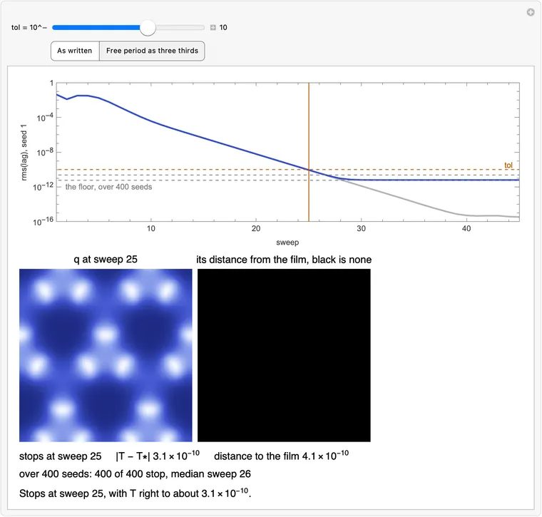
      

      Download ff-rate.wl

      The frame on the plane and one part of its rate as a size, each with a ring on a node, beside that node and its six neighbours as a labelled hexagon, with the arithmetic below and chips for diffusion, reaction or both.
      What this draws, in Wolfram 15.0, 00:02
      T -= np.clip(3 * np.sum(lag * speed) / np.sum(speed * speed), -0.1, 0.1)

      What: the one number that makes speed as close as possible to lag. It is a least-squares fit of a single number.

      Why: lag holds everything still wrong, and only part of that is timing. This reads off the part that looks like a timing error and ignores the rest, which is why it works on a messy field. How much of lag it explains is another matter, and the picture shows it.

      Try it: drag to make the right pane as dark as you can

      lag

      speed

      lag speed

      the expression rms(residual) left, squared lag, speed

      The fit, derived: why this quotient is the minimum

      Treat each field as one long list of numbers, with meaning np.sum(a * b): every node, both chemicals. Then the size of the residual is a parabola in :

      with the speed. Setting gives

      which is this piece of the line. At the residual is orthogonal to : the fit has taken all it can. What is left is

      and that is the dashed line on the chart, as a share of . So the cosine says how much of lag the number explains. The slider puts on a tick of its own, and on either side of it the residual is larger.

      np.sum rather than np.mean makes no difference to a quotient. The fit reads every node at once, so no one node's accident decides it; is one number and the fields hold 2592.

      How much of lag the number explains, measured

      On the film with off by : nearly all. 0.999983 at , 0.9998 at , 0.9983 at (find-film-modes.json, block m4_T_step). This lag is a copy of speed, which the first chip shows.

      In a run: little, at every stage. The median over seeds 1-200 is 0.277 at sweep 1 and between 0.11 and 0.36 through sweep 6 (find-film-runs.json, block page.early). Late in a run, once only the slow mode is left, it depends on where the frame sits on the loop: from 0.005 to 0.593, median 0.36, over seeds 5001-5400. The chips show seed 1 only, where it goes from at sweep 15 to at the end (find-film-extra-fix4.json): a value of that seed, not of the program.

      So the residual at the best stays near the whole of lag, even with the program well on its way. Most of lag is the slow mode, not timing. That the fit still reads something useful is the subject of the next card.

      The sign. Around the loop the signed cosine runs from -0.556 to 0.590, and passes through zero at two instants of each third of the loop ( is the time along the film from the exact frame), 0.112 and 0.293, where the slow mode leaves 's error alone. In a run its sign is the sign of 's error (find-film-modes.json, block m4b_cos_by_phase).

      Mathematica
      (* The T line's quotient as a fit of one number: lag, c x speed and what is left, with the size of what is left as a parabola in c, whose lowest point is exactly the expression. On the film it nearly reaches zero; in a run it barely dips. About 3 s on an M5. *)
      
      n = 36; box = 40.;   (* a triangular mesh of n x n nodes, in a repeating box of this side *)
      a = 1.; b = 2.3;     (* the Brusselator's constants; both chemicals diffuse at rate 1 *)
      dt = 0.02;           (* the longest time step *)
      
      (* How fast the chemicals q = {u, v} are changing: diffusion plus reaction. *)
      laplacian[f_] := 2/(3 (box/n)^2) ListCorrelate[{{1, 1, 0}, {1, -6, 1}, {0, 1, 1}}, f, {2, 2}];
      rate[{u_, v_}] := {laplacian[u] + a - (b + 1) u + u^2 v, laplacian[v] + b u - u^2 v};
      
      (* Run time forward by t (fourth-order Runge-Kutta). *)
      simulate[q0_, t_] := Module[{q = q0, steps = Ceiling[t/dt], h, k1, k2, k3, k4},
         h = t/steps;
         Do[
          k1 = rate[q];
          k2 = rate[q + h/2 k1];
          k3 = rate[q + h/2 k2];
          k4 = rate[q + h k3];
          q += h/6 (k1 + 2 k2 + 2 k3 + k4),
          {steps}];
         q];
      
      (* Slide the picture by a third of the box. On the film this costs T/3 of time. *)
      slide[q_] := RotateLeft[q, {0, n/3, 2 n/3}];
      
      (* Turn the picture 120 degrees about the origin. On the film this costs no time. *)
      turn[q_] := Table[f[[Mod[x - y, n] + 1, Mod[-y, n] + 1]], {f, q}, {y, 0, n - 1}, {x, 0, n - 1}];
      
      (* One frame of the film, its period T, and the number of sweeps it took. *)
      findFilm[q0_, T0_ : 6.355, tol_ : 1*^-10] := Module[{q, T = T0, third, twoThirds, lag, speed},
         q = (q0 + turn[q0] + turn[turn[q0]])/3;    (* costs no time, so impose it once and it stays *)
         Do[
          q = simulate[q, T];                       (* one free period: what decays, decays *)
          third = simulate[q, T/3];
          twoThirds = simulate[third, T/3];
      
          lag = slide[third] - q;                   (* zero on the film *)
          If[RootMeanSquare[Flatten[lag]] < tol, Return[{q, T, sweep}, Module]];
      
          (* T is off by 3 x lag / speed. Move it gently, since at first it's all noise. *)
          speed = rate[q];
          T -= Clip[3 Total[lag speed, 3]/Total[speed speed, 3], {-0.1, 0.1}];
      
          (* What obeys the rule survives the average; what ticks in unison cancels. *)
          q = (q + slide[third] + slide[slide[twoThirds]])/3,
          {sweep, 399}];
         $Failed];
      
      (* Start from the rest state plus white noise, and find the film. *)
      rest = {ConstantArray[a, {n, n}], ConstantArray[b/a, {n, n}]};
      noise[s_, amp_ : 0.1] := (SeedRandom[s]; rest + RandomVariate[NormalDistribution[0, amp], {2, n, n}]);
      
      (* Four points a mesh step, linear on the mesh's own triangles, as the page paints: a turned field then draws as the turned picture. *)
      meshTent = Table[Max[0., 1. - Max[Abs[i], Abs[j], Abs[i - j]]/4.], {j, -3, 3}, {i, -3, 3}];
      meshFine[f_] := ListCorrelate[meshTent, KroneckerProduct[f, Normal[SparseArray[{{1, 1} -> 1.}, {4, 4}]]], {4, 4}];
      
      {prjFrame, prjT, prjSweeps} = findFilm[noise[1]];
      
      (* The first 15 sweeps of findFilm's loop, keeping lag and speed at each. *)
      prjSweep = Module[{q = noise[1], T = 6.355, third, twoThirds, lag, speed},
         q = (q + turn[q] + turn[turn[q]])/3;
         Table[
          q = simulate[q, T];
          third = simulate[q, T/3];
          twoThirds = simulate[third, T/3];
          lag = slide[third] - q;
          speed = rate[q];
          T -= Clip[3 Total[lag speed, 3]/Total[speed speed, 3], {-0.1, 0.1}];
          q = (q + slide[third] + slide[slide[twoThirds]])/3;
          {lag, speed},
          15]];
      
      (* The four cases: lag and speed, on the film with T too long by 0.1, and in the run. *)
      prjCases = <|
         "On the film, T off by 0.1" -> {slide[simulate[prjFrame, (prjT + 0.1)/3]] - prjFrame, rate[prjFrame]},
         "Run, sweep 1" -> prjSweep[[1]], "Sweep 6" -> prjSweep[[6]], "Sweep 15" -> prjSweep[[15]]|>;
      
      (* The line's expression, the best c. *)
      prjBest[{lag_, speed_}] := Total[lag speed, 3]/Total[speed speed, 3];
      prjCos[{lag_, speed_}] := Total[lag speed, 3]/Sqrt[Total[lag lag, 3] Total[speed speed, 3]];
      (* What is left of lag squared, as a share, at c = v times the expression. *)
      prjLeft[cs_, v_] := With[{r = cs[[1]] - v prjBest[cs] cs[[2]]}, Total[r r, 3]/Total[cs[[1]] cs[[1]], 3]];
      
      (* A field's size at each node, both chemicals, as a picture: black is zero, white is hi. The same map as picture. *)
      prjGrey[{u_, v_}, hi_] := Image[Quiet[
          ImageTransformation[Image[Clip[Reverse[Sqrt[meshFine[u]^2 + meshFine[v]^2]]/hi, {0., 1.}]],
           {#[[1]] + #[[2]]/Sqrt[3.], 2 #[[2]]/Sqrt[3.]}/box + 0.5/(4 n) &, {200, 200},
           DataRange -> {{0, 1}, {0, 1}}, PlotRange -> {{-40., 40.}, {-40., 40.}},
           Padding -> "Periodic", Resampling -> "Linear"],
          RemoveAlphaChannel::imginv], ImageSize -> 200];
      
      Manipulate[
       With[{cs = prjCases[case], c = v prjBest[prjCases[case]]},
        With[{hi = Max[Sqrt[cs[[1, 1]]^2 + cs[[1, 2]]^2]], floor = 1 - prjCos[cs]^2},
         Column[{
           Grid[{{
              Labeled[prjGrey[cs[[1]], hi], "lag", Top],
              Labeled[prjGrey[c cs[[2]], hi], "c \[Times] speed", Top],
              Labeled[prjGrey[cs[[1]] - c cs[[2]], hi], "lag - c \[Times] speed", Top]}}],
           Plot[1 - 2 w prjCos[cs]^2 + w^2 prjCos[cs]^2, {w, 0, 2}, PlotRange -> {0, 1.12}, Frame -> True,
            FrameLabel -> {"c, as a multiple of the expression", "left of lag, squared"}, ImageSize -> 620, AspectRatio -> 0.25,
            PlotStyle -> RGBColor[0.2, 0.3, 0.8],
            Epilog -> {{RGBColor[0.75, 0.35, 0.], Dashed, Line[{{0, floor}, {2, floor}}], Text["least possible: " <> ToString[NumberForm[floor, 3]], {1.75, floor}, {0, -1.2}]},
              {RGBColor[0.75, 0.35, 0.], Line[{{v, 0}, {v, 1.12}}], PointSize[Medium], Point[{v, prjLeft[cs, v]}]}}],
           Row[{"the expression ", ScientificForm[prjBest[cs], 3], "     c ", ScientificForm[c, 3], "     rms(residual) ", ScientificForm[RootMeanSquare[Flatten[cs[[1]] - c cs[[2]]]], 3],
             "     left, squared ", PercentForm[prjLeft[cs, v], 3], "     cos(lag, speed) ", NumberForm[prjCos[cs], 4]}],
           Which[
            case === First[Keys[prjCases]] && v == 1, "At the expression the residual is black: this lag was a copy of speed, and one number holds all of it.",
            case === First[Keys[prjCases]], "Drag c: the residual darkens as c \[Times] speed takes up lag.",
            v == 1, "At the expression the residual is as dark as it gets, and it is nearly the same picture: most of this lag is not a timing error at all.",
            True, "Drag c: no value clears the residual. It only reads the part of lag that lies along speed."],
           "All three panes: size at each node, both chemicals, black is zero, white the largest of lag."
           }, Spacings -> 0.8]]],
       {{v, 1/2, "c, as a multiple of the expression"}, 0, 2, 1/40, Appearance -> "Labeled"},
       {{case, First[Keys[prjCases]], ""}, Keys[prjCases], ControlType -> SetterBar},
       BaseStyle -> {FontFamily -> "Helvetica"}, SaveDefinitions -> True]
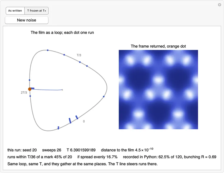
      

      Download ff-project.wl

      lag, c times speed and what is left, as sizes, over a parabola of what is left against c whose lowest point is the expression, with a slider for c and chips for the film and three sweeps of a run.
      What this draws, in Wolfram 15.0, 00:03
      # T is off by 3 x lag / speed. Move it gently, since at first it's all noise.
      T -= np.clip(3 * np.sum(lag * speed) / np.sum(speed * speed), -0.1, 0.1)

      What: from the last card is multiplied by 3 to turn it into a step for . On the exact film that step is the whole error in , up to a term in .

      Why: third is run for , so if is off by it is out of step by only , and that is what lag records. In a real run the comment is too simple: the step takes off about 0.57 of the error, because the rest of the field writes a new error each sweep.

      Try it: set the error , then apply the step

      lag

      speed

      reads error after

      The same step in the real run

      late step / error from 's own error -from q -together -

      On the film: the derivation, and how exact it is

      Write for simulate, for slide, for rate, for an exact frame and for the true period. The film's rule is . With , and since commutes with ,

      so by the expansion of

      So 's error after one step is about : the error is squared, as the button shows. In the table (exact frame; find-film-modes.json, block m4_T_step), 0.6405:

      step 1.0001071.00111.00321.01050.98911.02990.9666
      error after

      The step is still within about 3% of at , three times the largest step the clip allows. The sign of changes little, because the error after is second order.

      Caveat: is not one number. It is at the frame being read, and it runs from -1.28 to 0.64 around the loop. 0.6405 is its value at this frame, nearly its largest. So the sign of the error after can go either way: with the time along the film from the exact frame, at with it is , against the formula's . And a real sweep reads it after a free period, at a different frame: at it comes out , not (block m4c_kappa_and_sign). The card's own table reads a frame directly.

      The picture's triangle is one node of this: run , rise lag, slope speed. The node shown is where speed is largest.

      In the run: why about 0.57, not 1

      Linearise one whole sweep about the film, on the pair (field, ). With , , the average, and (the neutral mode), so :

      the last card's fit, on the lag that makes.

      The terms cancel. 's new error does not depend on its old one: on its own the step takes off exactly all of it, and is slaved to the field. For a mode of with factor , 's error shrinks with that mode, . So the step per unit of error is :

      Measured on the real linearised program: from itself 1.000000, from the field -0.428443 (find-film-modes.json, block m4_T_step.pair).

      The test. Late in a run the step over 's error is 0.5709 at the median of 400 seeds, 0.565 to 0.581 from 10% to 90% (find-film-runs.json). Re-read the same frame with at and what is left comes from the field alone, which is what the button does at sweep 18. Over seeds 1-5, 39 sweeps with rms(lag) from to : from 's own error 1.000000 (from 0.999992 to 1.000001), from the field -0.414 (from -0.502 to -0.334), which at this window still holds a share of faster modes (find-film-extra-D.json, block split).

      What this does not say. The chart's early sweeps are not a law: the step is clipped there and the field is not on the film. Nor is the 0.57 a slowness in that holds the run back: 's error simply falls with the slow mode, and with frozen at the run takes the same sweeps (the card on T -=).

      Mathematica
      (* The 3 in the T line: on the film with T off by delta, one node's time trace shows the T/3 tick missing by delta/3, so the projection reads delta/3 and 3 times it is delta; a button applies the step, and the error goes to about delta^2. Below, the same step in the real run takes off about 0.57 of the error. About 6 s on an M5. *)
      
      n = 36; box = 40.;   (* a triangular mesh of n x n nodes, in a repeating box of this side *)
      a = 1.; b = 2.3;     (* the Brusselator's constants; both chemicals diffuse at rate 1 *)
      dt = 0.02;           (* the longest time step *)
      
      (* How fast the chemicals q = {u, v} are changing: diffusion plus reaction. *)
      laplacian[f_] := 2/(3 (box/n)^2) ListCorrelate[{{1, 1, 0}, {1, -6, 1}, {0, 1, 1}}, f, {2, 2}];
      rate[{u_, v_}] := {laplacian[u] + a - (b + 1) u + u^2 v, laplacian[v] + b u - u^2 v};
      
      (* Run time forward by t (fourth-order Runge-Kutta). *)
      simulate[q0_, t_] := Module[{q = q0, steps = Ceiling[t/dt], h, k1, k2, k3, k4},
         h = t/steps;
         Do[
          k1 = rate[q];
          k2 = rate[q + h/2 k1];
          k3 = rate[q + h/2 k2];
          k4 = rate[q + h k3];
          q += h/6 (k1 + 2 k2 + 2 k3 + k4),
          {steps}];
         q];
      
      (* Slide the picture by a third of the box. On the film this costs T/3 of time. *)
      slide[q_] := RotateLeft[q, {0, n/3, 2 n/3}];
      
      (* Turn the picture 120 degrees about the origin. On the film this costs no time. *)
      turn[q_] := Table[f[[Mod[x - y, n] + 1, Mod[-y, n] + 1]], {f, q}, {y, 0, n - 1}, {x, 0, n - 1}];
      
      (* Start from the rest state plus white noise, and find the film. *)
      rest = {ConstantArray[a, {n, n}], ConstantArray[b/a, {n, n}]};
      noise[s_, amp_ : 0.1] := (SeedRandom[s]; rest + RandomVariate[NormalDistribution[0, amp], {2, n, n}]);
      
      (* Four points a mesh step, linear on the mesh's own triangles, as the page paints: a turned field then draws as the turned picture. *)
      meshTent = Table[Max[0., 1. - Max[Abs[i], Abs[j], Abs[i - j]]/4.], {j, -3, 3}, {i, -3, 3}];
      meshFine[f_] := ListCorrelate[meshTent, KroneckerProduct[f, Normal[SparseArray[{{1, 1} -> 1.}, {4, 4}]]], {4, 4}];
      
      (* findFilm's loop, keeping each sweep. With thirds, the free period is three thirds, so every step has one length and the run goes on down to the exact frame. *)
      thrRun[q0_, thirds_, sweeps_] := Module[{q = (q0 + turn[q0] + turn[turn[q0]])/3, T = 6.355, third, twoThirds, lag, speed, raw, row},
         Table[
          q = If[thirds, Nest[simulate[#, T/3] &, q, 3], simulate[q, T]];
          third = simulate[q, T/3];
          twoThirds = simulate[third, T/3];
          lag = slide[third] - q;
          speed = rate[q];
          raw = 3 Total[lag speed, 3]/Total[speed speed, 3];
          row = <|"q" -> q, "T" -> T, "speed" -> speed, "raw" -> raw|>;
          T -= Clip[raw, {-0.1, 0.1}];
          q = (q + slide[third] + slide[slide[twoThirds]])/3;
          row,
          sweeps]];
      
      (* The exact frame and the true period T*. *)
      {thrFrame, thrTstar} = Last[thrRun[noise[1], True, 45]] /@ {"q", "T"};
      thrSpeed = rate[thrFrame];
      
      (* With T = T* + delta: the lag, and the step the line would take. *)
      thrLag[delta_] := slide[simulate[thrFrame, (thrTstar + delta)/3]] - thrFrame;
      thrStep[delta_] := 3 Total[thrLag[delta] thrSpeed, 3]/Total[thrSpeed thrSpeed, 3];
      
      (* One node, where speed is largest: slide(q(t)) there for t around T*/3. It crosses the frame's own value at T*/3. *)
      thrNode = First[Position[Abs[thrSpeed[[1]]], Max[Abs[thrSpeed[[1]]]]]];
      thrAtNode[f_] := f[[1, Sequence @@ thrNode]];
      thrTrace = Module[{f = simulate[thrFrame, thrTstar/3 - 0.12]},
         Table[With[{v = thrAtNode[slide[f]]}, f = simulate[f, 0.008]; {w, v}], {w, -0.12, 0.12, 0.008}]];
      
      (* The real run, seed 1: the raw step over T's error, late about 1 - f, with f the factor a sweep of rms(lag). *)
      thrRows = thrRun[noise[1], False, 24];
      thrRatio = Table[{s, thrRows[[s, "raw"]]/(thrRows[[s, "T"]] - thrTstar)}, {s, 2, 24}];
      thrSlow = (RootMeanSquare[Flatten[slide[simulate[thrRows[[20, "q"]], thrRows[[20, "T"]]/3]] - thrRows[[20, "q"]]]]/
           RootMeanSquare[Flatten[slide[simulate[thrRows[[14, "q"]], thrRows[[14, "T"]]/3]] - thrRows[[14, "q"]]]])^(1/6);
      (* Sweep 18 split: the same frame re-read with T at T*, so what is left comes from q alone. *)
      thrSplit = With[{r = thrRows[[18]], q = thrRows[[18, "q"]]},
         With[{err = r["T"] - thrTstar, fromQ = 3 Total[(slide[simulate[q, thrTstar/3]] - q) r["speed"], 3]/Total[r["speed"] r["speed"], 3]},
          <|"late" -> r["raw"]/err, "fromT" -> (r["raw"] - fromQ)/err, "fromQ" -> fromQ/err|>]];
      
      (* A field's size as a picture: black is zero, white is hi. The same map as picture. *)
      thrGrey[u_, hi_] := Image[Quiet[
          ImageTransformation[Image[Clip[Reverse[Abs[meshFine[u]]]/hi, {0., 1.}]],
           {#[[1]] + #[[2]]/Sqrt[3.], 2 #[[2]]/Sqrt[3.]}/box + 0.5/(4 n) &, {220, 220},
           DataRange -> {{0, 1}, {0, 1}}, PlotRange -> {{-40., 40.}, {-40., 40.}},
           Padding -> "Periodic", Resampling -> "Linear"],
          RemoveAlphaChannel::imginv], ImageSize -> 220];
      
      (* The node's trace with the triangle: run delta/3, rise lag, slope speed. *)
      thrPlot[delta_] := With[{own = thrAtNode[thrFrame], run = delta/3, at = thrAtNode[slide[simulate[thrFrame, (thrTstar + delta)/3]]]},
         ListLinePlot[thrTrace, PlotStyle -> RGBColor[0.2, 0.3, 0.8], Frame -> True, ImageSize -> 340, AspectRatio -> 0.75, PlotRange -> All,
          FrameLabel -> {"time after T*/3", "slide(q(t)) at one node, u"},
          Epilog -> {
            {Dashed, Gray, Line[{{-0.12, own}, {0.12, own}}], Text["q at that node", {-0.08, own}, {0, -1}]},
            {Opacity[0.25], RGBColor[1., 0.69, 0.], Polygon[{{0, own}, {run, own}, {run, at}}]},
            {RGBColor[0.75, 0.35, 0.], Thick, Line[{{0, own}, {run, own}, {run, at}}], Text["\[Delta]/3", {run/2, own}, {0, 1.2}], Text["lag", {run, (own + at)/2}, {-1.5 Sign[run], 0}]},
            {Black, PointSize[Medium], Point[{0, own}]}, {RGBColor[0.75, 0.35, 0.], PointSize[Medium], Point[{run, at}]}}]];
      
      Manipulate[
       With[{d = If[Abs[delta] < 1*^-9, 1.*^-9, delta]},
        With[{lag = thrLag[d], step = thrStep[d]},
         With[{hi = If[Abs[d] < 2*^-9, 0.1, Max[Abs[lag[[1]]]]]},
          Column[{
            Grid[{{
               Labeled[thrGrey[lag[[1]], hi], "lag", Top],
               Labeled[thrGrey[d/3 thrSpeed[[1]], hi], "\[Delta]/3 \[Times] speed", Top],
               thrPlot[d]}}],
            Row[{"\[Delta] ", NumberForm[d, 4], "     \[Delta]/3 ", NumberForm[d/3, 4], "     c reads ", NumberForm[step/3, 4], "     3c ", NumberForm[step, 4], "     error after ", NumberForm[d - step, 3]}],
            If[history === {}, "Both panes: |u|, black is zero. The orange triangle has run \[Delta]/3, rise lag, and the curve's slope is speed.",
             Row[Riffle[NumberForm[#, 3] & /@ Append[history, d], " \[Rule] "], ""]],
            Style["The same step in the real run", Bold],
            ListLinePlot[thrRatio, Mesh -> All, MeshStyle -> PointSize[Small], PlotStyle -> RGBColor[0.2, 0.3, 0.8], Frame -> True, ImageSize -> 700, AspectRatio -> 0.22, PlotRange -> {{2, 24}, {-1, 4}},
             FrameLabel -> {"sweep of the run, seed 1", "raw step / T's error"},
             Epilog -> {{Dashed, Gray, Line[{{2, 1}, {24, 1}}], Text["on the film: 1", {22.5, 1}, {0, -1}]},
               {Dashed, RGBColor[0.75, 0.35, 0.], Line[{{2, 1 - thrSlow}, {24, 1 - thrSlow}}], Text["1 - " <> ToString[NumberForm[thrSlow, 3]], {22.5, 1 - thrSlow}, {0, 2.2}]}}],
            Row[{"Sweep 18, the same frame re-read with T at T*: late step / error ", NumberForm[thrSplit["late"], 3], "     from T's own error ", NumberForm[thrSplit["fromT"], {4, 3}],
              "     from q ", NumberForm[thrSplit["fromQ"], 3]}]
            }, Spacings -> 0.8]]]],
       {{delta, 0.3, "T off by \[Delta]"}, -0.3, 0.3, 0.01, Appearance -> "Labeled"},
       {{history, {}}, ControlType -> None},
       Button["Apply the step", history = Take[Append[history, delta], -Min[3, Length[history] + 1]]; delta = delta - thrStep[If[Abs[delta] < 1*^-9, 1*^-9, delta]]],
       BaseStyle -> {FontFamily -> "Helvetica"}, SaveDefinitions -> True]
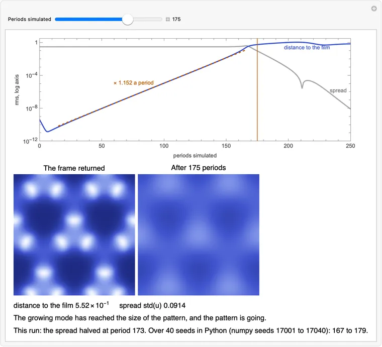
      

      Download ff-three.wl

      lag beside delta/3 times speed, and one node's time trace with the triangle of run delta/3, rise lag and slope speed; below, the raw step over T's error against the sweep, settling on 1 minus the slow factor rather than 1.
      What this draws, in Wolfram 15.0, 00:05
      # T is off by 3 x lag / speed. Move it gently, since at first it's all noise.
      T -= np.clip(3 * np.sum(lag * speed) / np.sum(speed * speed), -0.1, 0.1)

      What: however large the computed step, moves by at most in one sweep. It only fires in the first few sweeps.

      Why: at first the field is near rest, so speed is tiny and the quotient is large and meaningless. What the clip decides is narrow: any bound up to gives the film every time; with none, or a large one, a few runs in a hundred send to near zero and return a nearly uniform field with no error.

      Try it: move the bound, then try the noise that needs one

      fired largest raw largest sweeps ends

      What the clip decides: the table over 100 seeds at each bound

      Film means the run ended on the film, of 100 fresh seeds at each cell (seeds 6001-6100; find-film-runs.json, block page.clip). is the true period.

      boundfilm, noise noise noise median sweeps, noise largest , noise
      100100100450.041
      100100100260.095
      , as written100100100260.335
      100100100272.35
      999999276.39
      9810098274.07
      989899276.39
      989897276.39
      none989896276.39

      Read it this way. Up to : every run lands, 1200 of 1200 over the first four rows, and at bound no run's goes under 3.73. From up and with none: a few fail, 0 to 4 of 100 a cell, so what matters is having some bound, not this one. The sweeps barely move from up, so the clip does not speed the run. Only costs sweeps, for a dull reason: has to crawl the distance from at that rate. Started from with that bound a run takes 26 sweeps, against 48 from (20 seeds; the table's 45 is 100 others).

      The clip does change one more thing: where on the loop a run lands. At bound the landings bunch less, 0.34 against 0.65 as written (see the card on the return).

      Why the raw step is large at first: not noise so much as a small speed

      The quotient in the line, times 3, is

      with the speed. Medians of seeds 1-20 (find-film-extra-D.json, block early):

      sweep1246812
      rms(speed)0.0310.0270.1420.4570.5730.577
      rms(lag)0.0330.0100.0320.0200.0013
      0.300.160.170.350.120.19
      0.8780.1680.1100.0440.0008
      clip fired18 of 201511300

      At sweep 1 lag is already at its usual early size, but speed is far smaller than on the film (), since a field near rest barely moves. That small denominator is what makes the quotient large, with a modest cosine. So "all noise" in the comment overstates it: by then the first free period has cut most of the noise (its card), and what is left is a small field whose lag is not timing. As the field grows, speed grows, lag falls, and the clip stops firing.

      Over seeds 5001-5400: it fires in 1 to 8 sweeps per run, median 3, the last by sweep 9, and the raw step reaches 4.48.

      How a run with no bound fails, and what the failure looks like

      Not in one step. Over 8 failures of 300 (find-film-runs.json, block page.clip_no_bound), a run lasts 7 to 19 sweeps in all, with wandering first. Once falls far enough it is captured: a start at always ends with near 0 (20 of 20 from , and 19 of 20 at ; see the card on the guess). At bound no film run gets under 3.73, above that zone, which is why that bound is safe.

      The end is a kind of false success. A field that the slide leaves alone has lag , for small about , so the raw step is about and the step takes almost to zero at once. On the noise this card uses, seed 19 of the page's own generator, goes 6.355, 5.042, 1.788, 1.848, 0.059, 0.043, , and the run returns at sweep 8 with and a field nearly uniform, std() (find-film-extra-Dscan.json). With that small, lag is under tol whatever the field, and return looks like success. Bound on the same noise lands in 31 sweeps, and in 28. With no bound, 1 of the 8 failures ends the other way, nearly uniform at (the card on the raise).

      On this seed: this noise was picked for failing, 17 of the 19 seeds tried landed with no bound before the search stopped, which is a stop rule, not a rate. The rate is in the table above: 2 to 4 of 100.

      Mathematica
      (* The clip: the raw step per sweep against the bound, and T's trace, for each bound from 0.001 to none, on the noise of seed 1 and on a noise that needs a bound. Runs the real program at every setting, about 30 s on an M5, and scrubs what it recorded. *)
      
      n = 36; box = 40.;   (* a triangular mesh of n x n nodes, in a repeating box of this side *)
      a = 1.; b = 2.3;     (* the Brusselator's constants; both chemicals diffuse at rate 1 *)
      dt = 0.02;           (* the longest time step *)
      
      (* How fast the chemicals q = {u, v} are changing: diffusion plus reaction. *)
      laplacian[f_] := 2/(3 (box/n)^2) ListCorrelate[{{1, 1, 0}, {1, -6, 1}, {0, 1, 1}}, f, {2, 2}];
      rate[{u_, v_}] := {laplacian[u] + a - (b + 1) u + u^2 v, laplacian[v] + b u - u^2 v};
      
      (* Run time forward by t (fourth-order Runge-Kutta). *)
      simulate[q0_, t_] := Module[{q = q0, steps = Ceiling[t/dt], h, k1, k2, k3, k4},
         h = t/steps;
         Do[
          k1 = rate[q];
          k2 = rate[q + h/2 k1];
          k3 = rate[q + h/2 k2];
          k4 = rate[q + h k3];
          q += h/6 (k1 + 2 k2 + 2 k3 + k4),
          {steps}];
         q];
      
      (* Slide the picture by a third of the box. On the film this costs T/3 of time. *)
      slide[q_] := RotateLeft[q, {0, n/3, 2 n/3}];
      
      (* Turn the picture 120 degrees about the origin. On the film this costs no time. *)
      turn[q_] := Table[f[[Mod[x - y, n] + 1, Mod[-y, n] + 1]], {f, q}, {y, 0, n - 1}, {x, 0, n - 1}];
      
      (* Start from the rest state plus white noise, and find the film. *)
      rest = {ConstantArray[a, {n, n}], ConstantArray[b/a, {n, n}]};
      noise[s_, amp_ : 0.1] := (SeedRandom[s]; rest + RandomVariate[NormalDistribution[0, amp], {2, n, n}]);
      
      (* findFilm's loop with the bound as an argument, keeping each sweep. simulate cannot run a time that is not positive, so a T that has gone there holds q still. *)
      clpFlow[q_, t_] := If[t > 0, simulate[q, t], q];
      clpRun[s_, bound_] := Module[{q = noise[s], T = 6.355, third, twoThirds, lag, speed, raw, rms, rows = {}, status = "raised after 399 sweeps", sweeps = 0},
         q = (q + turn[q] + turn[turn[q]])/3;
         While[sweeps < 399,
          sweeps++;
          q = clpFlow[q, T];
          third = clpFlow[q, T/3];
          twoThirds = clpFlow[third, T/3];
          lag = slide[third] - q;
          rms = RootMeanSquare[Flatten[lag]];
          If[rms < 1*^-10, AppendTo[rows, <|"T" -> T, "raw" -> None|>]; status = "returned"; Break[]];
          speed = rate[q];
          raw = 3 Total[lag speed, 3]/Total[speed speed, 3];
          AppendTo[rows, <|"T" -> T, "raw" -> raw|>];
          T -= Clip[raw, {-bound, bound}];
          q = (q + slide[third] + slide[slide[twoThirds]])/3];
         <|"rows" -> rows, "T" -> T, "status" -> status, "spread" -> StandardDeviation[Flatten[q[[1]]]]|>];
      
      clpBounds = <|"0.001" -> 0.001, "0.01" -> 0.01, "0.1" -> 0.1, "1" -> 1., "2" -> 2., "4" -> 4., "none" -> Infinity|>;
      (* Seed 95 was picked for failing: with no bound, of seeds 1 to 124 here, seeds 78, 95 and 124 fail. *)
      clpNoises = <|"Noise of seed 1" -> 1, "A noise that needs a bound" -> 95|>;
      clpRuns = Association @@ Flatten[Table[{w, k} -> clpRun[clpNoises[w], clpBounds[k]], {w, Keys[clpNoises]}, {k, Keys[clpBounds]}]];
      clpTstar = clpRuns[{"Noise of seed 1", "0.1"}]["T"];
      
      (* Measured in Python over 100 seeds at each bound (numpy seeds 6001 to 6100): how many land on the film at noise 0.001, 0.1 and 1, and the median sweeps at noise 0.1. *)
      clpTable = <|"0.001" -> {100, 100, 100, 45}, "0.01" -> {100, 100, 100, 26}, "0.1" -> {100, 100, 100, 26}, "1" -> {100, 100, 100, 27},
         "2" -> {99, 99, 99, 27}, "4" -> {98, 98, 99, 27}, "none" -> {98, 98, 96, 27}|>;
      
      Manipulate[
       With[{r = clpRuns[{w, k}], bound = clpBounds[k]},
        With[{rows = r["rows"], raws = Cases[r["rows"], x_ /; NumericQ[x["raw"]] :> Abs[x["raw"]]]},
         With[{fired = Select[Transpose[{Range[Length[raws]], raws}], #[[2]] > bound &], worst = Max[Abs[#["T"] - clpTstar] & /@ rows]},
          Column[{
            ListLogPlot[Transpose[{Range[Length[raws]], raws}], Joined -> True, Mesh -> All, MeshStyle -> PointSize[Small], PlotStyle -> RGBColor[0.2, 0.3, 0.8], Frame -> True,
             FrameLabel -> {"sweep", "|raw step|, before the clip"}, ImageSize -> 640, AspectRatio -> 0.24, PlotRange -> {{1, Max[26, Length[rows]]}, {1*^-10, 10}},
             Epilog -> {If[bound < Infinity, {RGBColor[0.75, 0.35, 0.], Dashed, Line[{{0, Log[bound]}, {400, Log[bound]}}]}, {}],
               {RGBColor[0.75, 0.35, 0.], PointSize[Medium], Point[{#[[1]], Log[#[[2]]]} & /@ fired]}}],
            ListLinePlot[#["T"] & /@ rows, Mesh -> All, MeshStyle -> PointSize[Small], PlotStyle -> RGBColor[0.2, 0.3, 0.8],
             Frame -> True, FrameLabel -> {"sweep", "T, with T* dashed"}, ImageSize -> 640, AspectRatio -> 0.24, PlotRange -> All,
             Epilog -> {Directive[Gray, Dashed], Line[{{0, clpTstar}, {Max[26, Length[rows]], clpTstar}}]}],
            Row[{"bound ", k, "     fired ", Length[fired], "     largest raw ", NumberForm[Max[raws], 4], "     largest |T - T*| ", NumberForm[worst, 3], "     sweeps ", Length[rows], "     ends ",
              Which[Abs[r["T"] - clpTstar] < 1*^-6, "the film, T = " <> ToString[NumberForm[r["T"], 7]],
               r["status"] === "returned", Row[{"T = ", ScientificForm[r["T"], 3], ": a nearly uniform field, no error"}],
               True, r["status"]]}],
            Which[
             Abs[r["T"] - clpTstar] > 1*^-6, Row[{"T collapsed in ", Length[rows], " sweeps: the program returned a nearly uniform field, spread ", ScientificForm[r["spread"], 2], ", and raised nothing. The same noise lands at any bound up to 1."}],
             bound <= 0.001, "T crawls: it needs dozens of sweeps to cover the distance to T*, so the whole run waits for it.",
             fired =!= {}, Row[{"The bound fired in ", Length[fired], " sweeps, all early. The run lands."}],
             True, "The bound never fired: this run did not need it."],
            Row[{"Over 100 seeds at this bound, the film: ", clpTable[k][[1]], " at noise 0.001, ", clpTable[k][[2]], " at noise 0.1, ", clpTable[k][[3]], " at noise 1. Median sweeps ", clpTable[k][[4]], " at noise 0.1."}]
            }, Spacings -> 0.8]]]],
       {{k, "0.1", "The bound on T's step"}, Keys[clpBounds], ControlType -> Slider},
       {{w, "Noise of seed 1", ""}, Keys[clpNoises], ControlType -> SetterBar},
       BaseStyle -> {FontFamily -> "Helvetica"}, SaveDefinitions -> True]
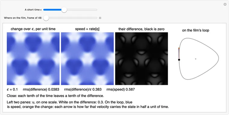
      

      Download ff-clip.wl

      The raw step per sweep on a log axis against the bound, with the fired sweeps orange, above T's trace against T*, with a slider for the bound and chips for the noise of seed 1 and a noise that needs a bound.
      What this draws, in Wolfram 15.0, 00:28
      T -= np.clip(3 * np.sum(lag * speed) / np.sum(speed * speed), -0.1, 0.1)

      What: the step comes off . This is the only line that changes .

      Why: if is too long, third has gone past the film's next frame, so lag lies along speed, the step is positive, and subtracting it brings down. This line does not set how fast the run converges, and the field finds the film's shape without it. What it gives is the period itself, without which the stop test can never fire.

      Try it: freeze , or flip the sign

      sweeps at the end rms(lag) at the end distance to the film

      Seed 1, the program's own noise. is the film's true period, which the program does not know.

      Why minus: the sign followed through, and what the other sign does

      With and , third is simulated longer than it should be, so it has moved further along the film: lag speed (the card on the 3). The projection is positive, the step about , and . If is too short everything changes sign together. Near the film, then, each step cancels the error.

      With T +=, each step adds the error instead: , until the clip limits it, and from then on moves a sweep: away from for about 50 sweeps, as far as 2.06, 11.26 and 11.36, and then back. On seeds 1-3 of numpy's generator, cut off at 60 sweeps as the chip is: 0 returned, ended between 2.86 and 10.35, and rms(lag) never fell below (find-film-extra-D.json, block flipped). Past that it was not followed.

      frozen: what the field finds anyway, and what it cannot do

      At : the same run. Frozen at against as written, sweeps on seeds 1, 2, 3: 25 and 25, 27 and 27, 26 and 26 (find-film-modes.json, block m4_T_step), and over 52 fresh seeds 36 are equal, the rest one sweep off. So 's line does not set the rate. The algebra agrees: the sweep on the pair (field, ) has the same factors as the sweep with frozen, plus a zero, because is slaved to the field.

      Off by : the program raises, every seed (10 of 10 at , so -0.0352; find-film-runs.json, block page.frozen_T). But rms(lag) does not settle at one level. At each sweep it is times rms(speed) at the current frame (0.997 to 1.006 of that). And the frame moves along the loop, by a sweep: in the free period, and on average in the slid frames. Measured -0.046874, predicted -0.046880. So as the frame goes round, speed changes, and rms(lag) rides between and , once in about 45 sweeps. The chart shows the start of this.

      It finds the film anyway. Three frames apart on a curved loop average to a point off it by , where is the film's acceleration. With rms() from 0.57 to 1.30 along the film, the formula gives 0.021 to 0.048 (find-film-extra-fix3.json). Measured after the average, ten seeds give 0.028 to 0.039 , and the chip's one frame, at the top of the range, 0.048 , which is (find-film-extra-D.json). So the shape arrives whatever is. What the frozen run lacks is closure: run for its own it misses by times rms(speed), and lag reads a third of that, so the stop test can never fire.

      It also picks where a run lands. With as written, 54.7% of 1000 runs land within of one of the three marks (, , ), against 16.7% if spread evenly. Frozen at they spread flat: 0.043 against 0.65. The reason is shown, not derived: the card on the return.

      What else this line can settle on

      The step is zero wherever the projection is zero, not only at . Starting from other , the same line ends elsewhere (seeds 14001-14020; find-film-runs.json, block page.start_T):

      • Near 0. From a start : a field the slide leaves alone, and walks down to zero. Returned, with no error (the clip's card).
      • and . The film's rule says on the film. It holds at , so at too. At the film turned by obeys it instead, to . At neither does, and there the uniform cycle wins.
      • the uniform cycle's period, . A nearly uniform field whose third has come round exactly once.

      So T=6.355 matters for which of these the run reaches: the card on the guess. And this line's new reaches the field only in the next sweep: the average below uses the frames already made with the old (the average's card).

      Mathematica
      (* The line T -= ... : T against sweep, with the true period dashed, and rms(lag) against sweep, for the program as written, T frozen at 6.355, T frozen at the true period, and the sign flipped. All four really run when this is evaluated, about 14 s on an M5; the buttons then switch between the runs. *)
      
      n = 36; box = 40.;   (* a triangular mesh of n x n nodes, in a repeating box of this side *)
      a = 1.; b = 2.3;     (* the Brusselator's constants; both chemicals diffuse at rate 1 *)
      dt = 0.02;           (* the longest time step *)
      
      (* How fast the chemicals q = {u, v} are changing: diffusion plus reaction. *)
      laplacian[f_] := 2/(3 (box/n)^2) ListCorrelate[{{1, 1, 0}, {1, -6, 1}, {0, 1, 1}}, f, {2, 2}];
      rate[{u_, v_}] := {laplacian[u] + a - (b + 1) u + u^2 v, laplacian[v] + b u - u^2 v};
      
      (* Run time forward by t (fourth-order Runge-Kutta). *)
      simulate[q0_, t_] := Module[{q = q0, steps = Ceiling[t/dt], h, k1, k2, k3, k4},
         h = t/steps;
         Do[
          k1 = rate[q];
          k2 = rate[q + h/2 k1];
          k3 = rate[q + h/2 k2];
          k4 = rate[q + h k3];
          q += h/6 (k1 + 2 k2 + 2 k3 + k4),
          {steps}];
         q];
      
      (* Slide the picture by a third of the box. On the film this costs T/3 of time. *)
      slide[q_] := RotateLeft[q, {0, n/3, 2 n/3}];
      
      (* Turn the picture 120 degrees about the origin. On the film this costs no time. *)
      turn[q_] := Table[f[[Mod[x - y, n] + 1, Mod[-y, n] + 1]], {f, q}, {y, 0, n - 1}, {x, 0, n - 1}];
      
      (* Start from the rest state plus white noise, and find the film. *)
      rest = {ConstantArray[a, {n, n}], ConstantArray[b/a, {n, n}]};
      noise[s_, amp_ : 0.1] := (SeedRandom[s]; rest + RandomVariate[NormalDistribution[0, amp], {2, n, n}]);
      
      (* findFilm with T's line changed: sign 1 is T -= as written, 0 freezes T, -1 is T +=. It keeps T and rms(lag) at every sweep, and stops at cap sweeps. *)
      ftmRun[sign_, T0_, cap_, tol_ : 1*^-10] := Module[{q0 = noise[1], q, T = T0, third, twoThirds, lag, speed, rows = {}},
         q = (q0 + turn[q0] + turn[turn[q0]])/3;
         Do[
          q = simulate[q, T];
          third = simulate[q, T/3];
          twoThirds = simulate[third, T/3];
          lag = slide[third] - q;
          AppendTo[rows, {T, RootMeanSquare[Flatten[lag]]}];
          If[Last[Last[rows]] < tol, Break[]];
          speed = rate[q];
          T -= sign Clip[3 Total[lag speed, 3]/Total[speed speed, 3], {-0.1, 0.1}];
          q = (q + slide[third] + slide[slide[twoThirds]])/3,
          {cap}];
         <|"T" -> rows[[All, 1]], "lag" -> rows[[All, 2]], "q" -> q|>];
      
      (* The film itself, from a tighter tol, as 48 frames round its loop, to measure a field's distance from: walk along it to the nearest point. *)
      ftmFilm = ftmRun[1, 6.355, 399, 3*^-11];
      ftmStar = Last[ftmFilm["T"]];    (* T*, the true period, which the program does not know *)
      ftmLoop = NestList[simulate[#, ftmStar/48] &, ftmFilm["q"], 47];
      ftmDistance[x_] := Module[{at = First[Ordering[RootMeanSquare[Flatten[x - #]] & /@ ftmLoop, 1]], t = ftmStar/48, from, f, v},
         from = ftmLoop[[Mod[at - 2, 48] + 1]];
         Do[f = simulate[from, t]; v = rate[f]; t += Total[(x - f) v, 3]/Total[v v, 3], {3}];
         RootMeanSquare[Flatten[simulate[from, t] - x]]];
      
      ftmCases = <|"written" -> ftmRun[1, 6.355, 399], "frozen" -> ftmRun[0, 6.355, 60], "star" -> ftmRun[0, ftmStar, 399], "flip" -> ftmRun[-1, 6.355, 60]|>;
      ftmFar = ftmDistance[#["q"]] & /@ ftmCases;
      
      ftmSay[which_] := With[{tail = MinMax[Drop[ftmCases[which]["lag"], 8]]}, <|
          "written" -> "As written: T settles on T* and rms(lag) falls through tol. The program returns.",
          "frozen" -> Row[{"T stays off, so lag never reaches tol: from sweep 9 it rides between ", ScientificForm[tail[[1]], 2], " and ", ScientificForm[tail[[2]], 2],
             " as the frame slides round the loop. The program would go on to sweep 399 and raise, yet the frame is already within ", ScientificForm[ftmFar["frozen"], 2], " of the film. Shown to sweep 60."}],
          "star" -> "T held at T*, which the program does not know: the same number of sweeps, or one off. So this line does not set the rate.",
          "flip" -> "With the sign flipped each step adds the error instead of taking it off. T walks away at the clip's rate, turning back only far from the film, and the frame is not on it. Shown to sweep 60."|>[which]];
      
      ftmView[which_] := Module[{c = ftmCases[which], sweeps},
         sweeps = Length[c["T"]];
         Style[Column[{
            Grid[{{
               ListLinePlot[c["T"], Mesh -> All, MeshStyle -> PointSize[0.012], PlotStyle -> RGBColor[0.19, 0.29, 0.78], GridLines -> {None, {{ftmStar, Directive[GrayLevel[0.35], Thick, Dashed]}}},
                PlotRange -> {{1, Max[sweeps, 28]}, MinMax[Append[c["T"], ftmStar], Scaled[0.08]]}, Frame -> True, FrameLabel -> {"sweep", None}, PlotLabel -> "T, with T* dashed", ImageSize -> 400, AspectRatio -> 0.6],
               ListLogPlot[{c["lag"], Table[1*^-10, Max[sweeps, 28]]}, Joined -> True, PlotStyle -> {RGBColor[0.19, 0.29, 0.78], Directive[RGBColor[0.75, 0.35, 0], Dashed]},
                PlotRange -> {{1, Max[sweeps, 28]}, If[which === "frozen", {0.001, 0.1}, {1*^-11, 1}]}, Frame -> True, FrameLabel -> {"sweep", None},
                PlotLabel -> If[which === "frozen", "rms(lag), a closer axis: tol is far below it", "rms(lag), with tol dashed"], ImageSize -> 400, AspectRatio -> 0.6]}}],
            Row[{"sweeps ", sweeps, "     T at the end ", NumberForm[Last[c["T"]], {7, 6}], "     rms(lag) at the end ", ScientificForm[Last[c["lag"]], 2], "     distance to the film ", ScientificForm[ftmFar[which], 2]}],
            Pane[ftmSay[which], 800]}, Spacings -> 0.7], FontFamily -> "Helvetica", 12]];
      
      Manipulate[ftmView[ftmWhich],
       {{ftmWhich, "written", "How T is treated"}, {"written" -> "As written", "frozen" -> "T frozen at 6.355", "star" -> "T frozen at T*", "flip" -> "T += instead"}, ControlType -> SetterBar},
       SaveDefinitions -> True]
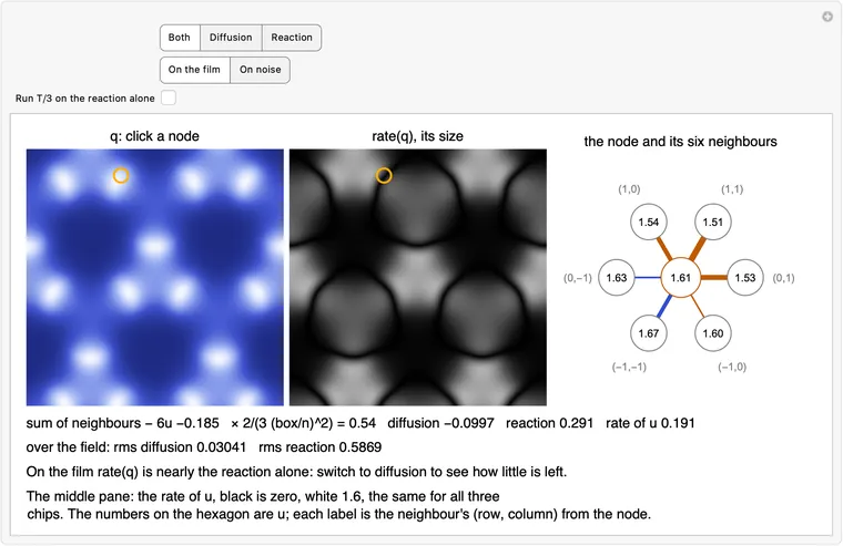
      

      Download ff-tminus.wl

      T against sweep with the true period dashed, and rms(lag) on a log axis falling through tol, with buttons for T frozen at 6.355, T frozen at the true period, and the sign flipped.
      What this draws, in Wolfram 15.0, 00:13

      24. The average

      q = (q + slide(third) + slide(slide(two_thirds))) / 3

      What: two_thirds is ahead of q, so it is slid back twice. third is only ahead, so it is slid once.

      Why: one slide undoes of time, and frames can only be averaged once they show the same picture. Two slides, and two_thirds lands exactly on q.

      Try it: slide two_thirds 0, 1, 2 or 3 times

      q, the exact film

      the difference, black is zero

      on the film's loop

      rms(difference)

      Why exactly two, and why three adds nothing

      Write for simulate and for slide. The film's rule at the frame is . The slide commutes with the simulation, bit for bit (difference 0; find-film-modes.json, block m2_commute), so

      Measured on the exact frame, in Python, rms of slide applied times to two_thirds, minus q: gives 0.6617, gives 0.6617, gives , and is again (find-film-extra-E.json). Those two large numbers are equal because the three frames are a slide apart, and a slide does not change a distance.

      Three slides are the identity: exactly, since the slide moves by and three of those are whole boxes (difference 0). So is one slide the other way, and the two-slide form in the code is only for reading. A fourth frame, at , would need three slides, that is none: it would be the next free period's frame, with nothing new about the film.

      On the loop picture each slide is a rotation by of the loop's plane, measured as -120.0° (find-film-modes.json, block m6_state_space). The dot is exact: it is the frame's own projection.

      In a run the frames do not line up yet: that is the point

      The black pane is the exact film. In a run, after the slides, slide(slide(two_thirds)) differs from q by 0.0850, rms, on sweep 4 of seed 1, and the misfit falls with the run. Late in the run the two misfits keep a fixed ratio: rms(slide(slide(two_thirds)) - q) over rms(slide(third) - q) is 1.814 at sweep 24, near the 1.806 of the slow mode, since for a mode the two differences are and . The next card shows the frames themselves.

      Mathematica
      (* slide[slide[twoThirds]]: two thirds of a period later, slid 0, 1, 2 or 3 times. Beside the film's frame q: the slid frame, their difference (black is zero), and where the slid frame sits on the film's loop. Only two slides land on q. An orange ring marks the same place in both frames. Evaluates in about 2 s on an M5. *)
      
      n = 36; box = 40.;   (* a triangular mesh of n x n nodes, in a repeating box of this side *)
      a = 1.; b = 2.3;     (* the Brusselator's constants; both chemicals diffuse at rate 1 *)
      dt = 0.02;           (* the longest time step *)
      
      (* How fast the chemicals q = {u, v} are changing: diffusion plus reaction. *)
      laplacian[f_] := 2/(3 (box/n)^2) ListCorrelate[{{1, 1, 0}, {1, -6, 1}, {0, 1, 1}}, f, {2, 2}];
      rate[{u_, v_}] := {laplacian[u] + a - (b + 1) u + u^2 v, laplacian[v] + b u - u^2 v};
      
      (* Run time forward by t (fourth-order Runge-Kutta). *)
      simulate[q0_, t_] := Module[{q = q0, steps = Ceiling[t/dt], h, k1, k2, k3, k4},
         h = t/steps;
         Do[
          k1 = rate[q];
          k2 = rate[q + h/2 k1];
          k3 = rate[q + h/2 k2];
          k4 = rate[q + h k3];
          q += h/6 (k1 + 2 k2 + 2 k3 + k4),
          {steps}];
         q];
      
      (* Slide the picture by a third of the box. On the film this costs T/3 of time. *)
      slide[q_] := RotateLeft[q, {0, n/3, 2 n/3}];
      
      (* Turn the picture 120 degrees about the origin. On the film this costs no time. *)
      turn[q_] := Table[f[[Mod[x - y, n] + 1, Mod[-y, n] + 1]], {f, q}, {y, 0, n - 1}, {x, 0, n - 1}];
      
      (* One frame of the film, its period T, and the number of sweeps it took. *)
      findFilm[q0_, T0_ : 6.355, tol_ : 1*^-10] := Module[{q, T = T0, third, twoThirds, lag, speed},
         q = (q0 + turn[q0] + turn[turn[q0]])/3;    (* costs no time, so impose it once and it stays *)
         Do[
          q = simulate[q, T];                       (* one free period: what decays, decays *)
          third = simulate[q, T/3];
          twoThirds = simulate[third, T/3];
      
          lag = slide[third] - q;                   (* zero on the film *)
          If[RootMeanSquare[Flatten[lag]] < tol, Return[{q, T, sweep}, Module]];
      
          (* T is off by 3 x lag / speed. Move it gently, since at first it's all noise. *)
          speed = rate[q];
          T -= Clip[3 Total[lag speed, 3]/Total[speed speed, 3], {-0.1, 0.1}];
      
          (* What obeys the rule survives the average; what ticks in unison cancels. *)
          q = (q + slide[third] + slide[slide[twoThirds]])/3,
          {sweep, 399}];
         $Failed];
      
      (* Start from the rest state plus white noise, and find the film. *)
      rest = {ConstantArray[a, {n, n}], ConstantArray[b/a, {n, n}]};
      noise[s_, amp_ : 0.1] := (SeedRandom[s]; rest + RandomVariate[NormalDistribution[0, amp], {2, n, n}]);
      
      (* Four points a mesh step, linear on the mesh's own triangles, as the page paints: a turned field then draws as the turned picture. *)
      meshTent = Table[Max[0., 1. - Max[Abs[i], Abs[j], Abs[i - j]]/4.], {j, -3, 3}, {i, -3, 3}];
      meshFine[f_] := ListCorrelate[meshTent, KroneckerProduct[f, Normal[SparseArray[{{1, 1} -> 1.}, {4, 4}]]], {4, 4}];
      
      (* A field on the plane, as a picture: the mesh's two axes are 120 degrees apart. Blue is lo, white is hi. *)
      picture[u_, {lo_, hi_}, size_ : 240] := Colorize[
         Quiet[    (* Wolfram 15's ImageTransformation trips on the notebook's light/dark background, harmlessly *)
          ImageTransformation[Image[Rescale[Reverse[meshFine[u]], {lo, hi}]],
           {#[[1]] + #[[2]]/Sqrt[3.], 2 #[[2]]/Sqrt[3.]}/box + 0.5/(4 n) &, {size, size},
           DataRange -> {{0, 1}, {0, 1}}, PlotRange -> {{-40., 40.}, {-40., 40.}},
           Padding -> "Periodic", Resampling -> "Linear"],
          RemoveAlphaChannel::imginv],
         ColorFunction -> (Blend[{RGBColor[0.118, 0.165, 0.51], RGBColor[0.251, 0.329, 0.808], RGBColor[0.588, 0.667, 0.941], RGBColor[0.961, 0.973, 1.]}, #] &), ColorFunctionScaling -> False];
      
      {fs2Q, fs2T, fs2Sweeps} = findFilm[noise[1]];
      fs2Two = simulate[simulate[fs2Q, fs2T/3], fs2T/3];
      fs2Range = MinMax[fs2Q[[1]]];
      fs2Slid[k_] := Nest[slide, fs2Two, k];
      
      (* The film's loop: 48 frames round it, in the plane of their first two principal components. *)
      fs2Loop = Flatten /@ NestList[simulate[#, fs2T/48] &, fs2Q, 47];
      fs2Mean = Mean[fs2Loop];
      fs2Axes = Transpose[Last[SingularValueDecomposition[# - fs2Mean & /@ fs2Loop, 2]]];
      fs2Project[q_] := fs2Axes.(Flatten[q] - fs2Mean);
      
      (* The ring: u's brightest node of q, at its copy nearest the middle of the picture. Mesh node (x, y) sits at (x - y/2, y Sqrt[3]/2) box/n; the picture spans -40 to 40 over 240 pixels. *)
      fs2Spot = With[{at = First[Position[fs2Q[[1]], Max[fs2Q[[1]]]]] - 1},
         First[MinimalBy[Flatten[Table[({at[[2]] + i n - (at[[1]] + j n)/2, (at[[1]] + j n) Sqrt[3.]/2}) box/n, {i, -2, 2}, {j, -2, 2}], 1], Norm]]];
      fs2Ringed[u_] := Show[picture[u, fs2Range], Graphics[{{Black, Thickness[0.02], Circle[(fs2Spot + 40)/80 240, 13]}, {RGBColor[1, 0.69, 0], Thickness[0.012], Circle[(fs2Spot + 40)/80 240, 13]}}], ImageSize -> 180];
      
      (* The difference, black is zero, white is 1.5: picture's mapping in grey. *)
      fs2Grey[u_] := Show[Quiet[
          ImageTransformation[Image[Clip[Abs[Reverse[meshFine[u]]]/1.5, {0, 1}]],
           {#[[1]] + #[[2]]/Sqrt[3.], 2 #[[2]]/Sqrt[3.]}/box + 0.5/(4 n) &, {240, 240},
           DataRange -> {{0, 1}, {0, 1}}, PlotRange -> {{-40., 40.}, {-40., 40.}},
           Padding -> "Periodic", Resampling -> "Linear"],
          RemoveAlphaChannel::imginv], ImageSize -> 180];
      
      fs2LoopPlot[f_] := ListLinePlot[Append[#, First[#]] &[fs2Axes.(# - fs2Mean) & /@ fs2Loop], PlotStyle -> Directive[Gray, Thick], AspectRatio -> 1, Axes -> False, ImageSize -> 180, PlotRangePadding -> Scaled[0.08],
         Epilog -> {{Gray, Thick, Line[{fs2Project[rest] - {4, 0}, fs2Project[rest] + {4, 0}}], Line[{fs2Project[rest] - {0, 4}, fs2Project[rest] + {0, 4}}]},
           {RGBColor[0.19, 0.29, 0.78], PointSize[0.05], Point[fs2Project[fs2Q]]}, {RGBColor[0.75, 0.35, 0], PointSize[0.035], Point[fs2Project[f]]}}];
      
      fs2Name = {"twoThirds", "slide[twoThirds]", "slide[slide[twoThirds]]", "slide[slide[slide[twoThirds]]]"};
      fs2Say = {"Not slid at all: the picture is two thirds of a period ahead of q, and nothing matches.", "One slide takes off T/3. It is still T/3 ahead, the same distance from q.",
         "Two slides take off 2T/3: the same picture as q, down to the tolerance findFilm stopped at. Now it can be averaged with q.", "Three slides are whole boxes, so this is the unslid frame again, bit for bit."};
      
      fs2View[k_] := Module[{f = fs2Slid[k], d},
         d = f - fs2Q;
         Style[Column[{
            Row[{Labeled[fs2Ringed[fs2Q[[1]]], "q, the film", Top], Labeled[fs2Ringed[f[[1]]], fs2Name[[k + 1]], Top], Labeled[fs2Grey[d[[1]]], "the difference, black is zero", Top], Labeled[fs2LoopPlot[f], "on the film's loop", Top]}, " "],
            Row[{"rms(difference) ", ScientificForm[RootMeanSquare[Flatten[d]], 2]}],
            fs2Say[[k + 1]]}, Spacings -> 0.7], FontFamily -> "Helvetica", 12]];
      
      Manipulate[fs2View[fs2K],
       {{fs2K, 2, "Slides of twoThirds"}, {0, 1, 2, 3}, ControlType -> SetterBar},
       SaveDefinitions -> True]
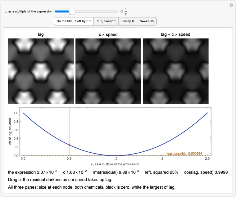
      

      Download ff-slide2.wl

      The film frame beside two thirds of a period later slid twice, the same bright spot ringed in both, an all-black difference, and the frame as a dot on the film's closed loop.
      What this draws, in Wolfram 15.0, 00:02
      q = (q + slide(third) + slide(slide(two_thirds))) / 3

      What: the three frames, lined up, are averaged, and the result is where the next sweep starts.

      Why: not to pick the best frame: the average is never the nearest of them to the film. It accepts that small loss because it cancels the mode that would otherwise grow. Without it, this program never finds the film.

      Try it: scrub the sweeps, then run it without this line

      q

      slide(third)

      slide(slide(two_thirds))

      the average

      avg - q, black is zero

      distance to the film: q the average nearest frame

      Why the average is not the nearest frame, and what it buys

      Take one mode with factor per third of a period. After the slides the three frames hold it as times its size in q, and the average as . For the mode that is left late in the run, 0.8059, real, so the frames sit at 0.8059 and 0.6495 and the average at 0.8185: farther out than either later frame. The chart reads 0.8043, 0.6485 and 0.8176 at sweep 24.

      In every sweep measured the average is farther from the film than the nearest of its three frames: it is nearer in 0 of 148 sweeps of seeds 1 to 6, rms distance to the nearest point of the exact orbit (find_film_extra_E.py). So "averaging removes error" is not what this line does on the mode that sets the pace; on that one it costs a little.

      What it buys is on the modes near . The frame slide(slide(two_thirds)) alone is a plain simulation, slid: it keeps the unison mode, and that grows 1.1608 times a period. By the sweep's end the average holds 0.0351 of it. The next three cards are about that.

      Without the line: what the program does, measured

      As in the demo, with the T step left on: walks down at the clip's rate, since a field does repeat if the wait is short enough, and first reaches at sweep 71 to 97 on seeds 1-20, 68 to 122 on seeds 9301-9340. Seed 1 here: sweep 85. Below that simulate hands q back unchanged, so the program runs on to sweep 399 and raises, on a field not uniform enough to stop.

      With frozen as well, it is a plain simulation with no average: the field goes to nearly uniform oscillation, 20 of 20 at and 20 of 20 at (find-film-runs.json).

      Small print: a jump, the old T, and the last sweep

      A jump. Any field is a state the equation can start from, but no simulation goes from q to the average. On sweep 4 it moves q by 0.0423, rms; late in a run by 0.189 of q's distance to the film. The free period at the top of the next sweep is the equation again, and it starts from this jump.

      The old . The line above has just changed , but this line does not read it: the three frames were made with the of this sweep's start. The new first acts on the next free period.

      On the film it does nothing. Applied to the exact frame, it moves it by . And the program's return is above this line, so the returned frame is q, made by simulate, not an average.

      Sweeps here. The scrubber stops one short of the last sweep, because that sweep returns before reaching this line. The distances come from a Python run of seed 1, the same noise as the page's fields.

      Mathematica
      (* The whole last line: the three frames and their average, sweep by sweep, and each frame's distance to the film as a share of q's. The average is never the nearest frame. A second button removes the line and really runs the program without it: T walks down to 0. Evaluates in about 8 s on an M5. *)
      
      n = 36; box = 40.;   (* a triangular mesh of n x n nodes, in a repeating box of this side *)
      a = 1.; b = 2.3;     (* the Brusselator's constants; both chemicals diffuse at rate 1 *)
      dt = 0.02;           (* the longest time step *)
      
      (* How fast the chemicals q = {u, v} are changing: diffusion plus reaction. *)
      laplacian[f_] := 2/(3 (box/n)^2) ListCorrelate[{{1, 1, 0}, {1, -6, 1}, {0, 1, 1}}, f, {2, 2}];
      rate[{u_, v_}] := {laplacian[u] + a - (b + 1) u + u^2 v, laplacian[v] + b u - u^2 v};
      
      (* Run time forward by t (fourth-order Runge-Kutta). *)
      simulate[q0_, t_] := Module[{q = q0, steps = Ceiling[t/dt], h, k1, k2, k3, k4},
         h = t/steps;
         Do[
          k1 = rate[q];
          k2 = rate[q + h/2 k1];
          k3 = rate[q + h/2 k2];
          k4 = rate[q + h k3];
          q += h/6 (k1 + 2 k2 + 2 k3 + k4),
          {steps}];
         q];
      
      (* Slide the picture by a third of the box. On the film this costs T/3 of time. *)
      slide[q_] := RotateLeft[q, {0, n/3, 2 n/3}];
      
      (* Turn the picture 120 degrees about the origin. On the film this costs no time. *)
      turn[q_] := Table[f[[Mod[x - y, n] + 1, Mod[-y, n] + 1]], {f, q}, {y, 0, n - 1}, {x, 0, n - 1}];
      
      (* One frame of the film, its period T, and the number of sweeps it took. *)
      findFilm[q0_, T0_ : 6.355, tol_ : 1*^-10] := Module[{q, T = T0, third, twoThirds, lag, speed},
         q = (q0 + turn[q0] + turn[turn[q0]])/3;    (* costs no time, so impose it once and it stays *)
         Do[
          q = simulate[q, T];                       (* one free period: what decays, decays *)
          third = simulate[q, T/3];
          twoThirds = simulate[third, T/3];
      
          lag = slide[third] - q;                   (* zero on the film *)
          If[RootMeanSquare[Flatten[lag]] < tol, Return[{q, T, sweep}, Module]];
      
          (* T is off by 3 x lag / speed. Move it gently, since at first it's all noise. *)
          speed = rate[q];
          T -= Clip[3 Total[lag speed, 3]/Total[speed speed, 3], {-0.1, 0.1}];
      
          (* What obeys the rule survives the average; what ticks in unison cancels. *)
          q = (q + slide[third] + slide[slide[twoThirds]])/3,
          {sweep, 399}];
         $Failed];
      
      (* Start from the rest state plus white noise, and find the film. *)
      rest = {ConstantArray[a, {n, n}], ConstantArray[b/a, {n, n}]};
      noise[s_, amp_ : 0.1] := (SeedRandom[s]; rest + RandomVariate[NormalDistribution[0, amp], {2, n, n}]);
      
      (* Four points a mesh step, linear on the mesh's own triangles, as the page paints: a turned field then draws as the turned picture. *)
      meshTent = Table[Max[0., 1. - Max[Abs[i], Abs[j], Abs[i - j]]/4.], {j, -3, 3}, {i, -3, 3}];
      meshFine[f_] := ListCorrelate[meshTent, KroneckerProduct[f, Normal[SparseArray[{{1, 1} -> 1.}, {4, 4}]]], {4, 4}];
      
      (* A field on the plane, as a picture: the mesh's two axes are 120 degrees apart. Blue is lo, white is hi. *)
      picture[u_, {lo_, hi_}, size_ : 240] := Colorize[
         Quiet[    (* Wolfram 15's ImageTransformation trips on the notebook's light/dark background, harmlessly *)
          ImageTransformation[Image[Rescale[Reverse[meshFine[u]], {lo, hi}]],
           {#[[1]] + #[[2]]/Sqrt[3.], 2 #[[2]]/Sqrt[3.]}/box + 0.5/(4 n) &, {size, size},
           DataRange -> {{0, 1}, {0, 1}}, PlotRange -> {{-40., 40.}, {-40., 40.}},
           Padding -> "Periodic", Resampling -> "Linear"],
          RemoveAlphaChannel::imginv],
         ColorFunction -> (Blend[{RGBColor[0.118, 0.165, 0.51], RGBColor[0.251, 0.329, 0.808], RGBColor[0.588, 0.667, 0.941], RGBColor[0.961, 0.973, 1.]}, #] &), ColorFunctionScaling -> False];
      
      (* The program, keeping what this line takes in and gives out at every sweep. The last sweep returns before reaching it. *)
      favRows = Module[{q0 = noise[1], q, T = 6.355, third, twoThirds, lag, speed, rows = {}},
         q = (q0 + turn[q0] + turn[turn[q0]])/3;
         Do[
          q = simulate[q, T];
          third = simulate[q, T/3];
          twoThirds = simulate[third, T/3];
          lag = slide[third] - q;
          If[RootMeanSquare[Flatten[lag]] < 1*^-10, Break[]];
          speed = rate[q];
          T -= Clip[3 Total[lag speed, 3]/Total[speed speed, 3], {-0.1, 0.1}];
          AppendTo[rows, {q, slide[third], slide[slide[twoThirds]], (q + slide[third] + slide[slide[twoThirds]])/3}];
          q = Last[Last[rows]],
          {399}];
         rows];
      favLast = Length[favRows];
      
      (* The same with the line really removed: q just carries on. T is kept until it first reaches 0; below that simulate does nothing, and the program would run on to sweep 399 and raise. *)
      favOff = Module[{q0 = noise[1], q, T = 6.355, third, lag, speed, Ts = {}},
         q = (q0 + turn[q0] + turn[turn[q0]])/3;
         While[T > 0 && Length[Ts] < 399,
          AppendTo[Ts, T];
          q = simulate[q, T];
          third = simulate[q, T/3];
          lag = slide[third] - q;
          speed = rate[q];
          T -= Clip[3 Total[lag speed, 3]/Total[speed speed, 3], {-0.1, 0.1}]];
         <|"T" -> Ts, "q" -> q|>];
      
      (* The film, from a tighter tol, as 48 frames round its loop. A field's distance to it: walk along the loop to the nearest point. *)
      {favFilm, favT, favSweeps} = findFilm[noise[1], 6.355, 3*^-11];
      favLoop = NestList[simulate[#, favT/48] &, favFilm, 47];
      favRange = MinMax[favFilm[[1]]];
      favDistance[x_] := Module[{at = First[Ordering[RootMeanSquare[Flatten[x - #]] & /@ favLoop, 1]], t = favT/48, from, f, v},
         from = favLoop[[Mod[at - 2, 48] + 1]];
         Do[f = simulate[from, t]; v = rate[f]; t += Total[(x - f) v, 3]/Total[v v, 3], {3}];
         RootMeanSquare[Flatten[simulate[from, t] - x]]];
      favFar = Map[favDistance, favRows, {2}];    (* at each sweep: q, slide[third], slide[slide[twoThirds]], the average *)
      
      (* The chart stops where the film's own error starts to show in the shares. *)
      favChart[sweep_] := Module[{ok = Select[Range[favLast], favFar[[#, 1]] > 2*^-9 &]},
         ListLinePlot[Table[Transpose[{ok, favFar[[ok, k]]/favFar[[ok, 1]]}], {k, {3, 2, 4}}],
          PlotStyle -> {Directive[Gray, Dashed], Gray, Directive[RGBColor[0.19, 0.29, 0.78], Thick]}, PlotRange -> {{1, Max[ok]}, {0.4, 1.05}},
          PlotLabels -> {"slide[slide[twoThirds]]", "slide[third]", "the average"}, GridLines -> {{{sweep, RGBColor[0.75, 0.35, 0]}}, {{1, Dashed}}},
          AxesLabel -> {"sweep", None}, PlotLabel -> "distance to the film, as a share of q's", ImageSize -> 720, AspectRatio -> 0.24]];
      
      favPane[u_, label_] := Labeled[Show[picture[u, favRange], ImageSize -> 140], label, Top];
      favDiffPane[u_, hi_] := Labeled[Show[Quiet[
           ImageTransformation[Image[Clip[Abs[Reverse[meshFine[u]]]/hi, {0, 1}]],
            {#[[1]] + #[[2]]/Sqrt[3.], 2 #[[2]]/Sqrt[3.]}/box + 0.5/(4 n) &, {240, 240},
            DataRange -> {{0, 1}, {0, 1}}, PlotRange -> {{-40., 40.}, {-40., 40.}},
            Padding -> "Periodic", Resampling -> "Linear"],
           RemoveAlphaChannel::imginv], ImageSize -> 140], "avg - q, black is zero", Top];
      
      favWritten[sweep_] := Module[{f = favRows[[sweep]], d = favFar[[sweep]], jump, hi, near},
         jump = f[[4]] - f[[1]]; hi = 3 RootMeanSquare[Flatten[jump]]; near = Min[Take[d, 3]];
         Column[{
           Row[{favPane[f[[1, 1]], "q"], favPane[f[[2, 1]], "slide[third]"], favPane[f[[3, 1]], "slide[slide[twoThirds]]"], favPane[f[[4, 1]], "the average"], favDiffPane[jump[[1]], hi]}, " "],
           favChart[sweep],
           Row[{"distance to the film: q ", ScientificForm[d[[1]], 3], "     the average ", ScientificForm[d[[4]], 3], "     nearest frame ", ScientificForm[near, 3]}],
           If[d[[4]] < near, "Here the average is the nearest.", Row[{"The average is not the nearest frame: it is ", NumberForm[d[[4]]/near, {3, 2}], " times as far as the nearest one."}]],
           Row[{"Colour: u on the film's own range. White on the right: ", ScientificForm[hi, 2], "."}]}, Spacings -> 0.7]];
      
      favWithout = Column[{
          Row[{favPane[favOff["q"][[1]], "q, with no average"],
            ListLinePlot[{Table[favT, Length[favOff["T"]]], favOff["T"]}, PlotStyle -> {Directive[Gray, Dashed], Directive[RGBColor[0.19, 0.29, 0.78], Thick]}, AxesLabel -> {"sweep", "T"},
             PlotLabel -> "T with no average; the film's T dashed", PlotRange -> {-0.5, 8}, ImageSize -> 560, AspectRatio -> 0.35]}, " "],
          "T reached 0 at sweep " <> ToString[Length[favOff["T"]]] <> ". A shorter wait always looks better: a field does repeat if the wait is short enough. Simulating for no time returns q unchanged, so the program would go on to sweep 399 and raise."}, Spacings -> 0.7];
      
      Manipulate[Style[If[favWhich === "written", favWritten[favSweep], favWithout], FontFamily -> "Helvetica", 12],
       {{favWhich, "written", "The program"}, {"written" -> "As written", "off" -> "Without this line"}, ControlType -> SetterBar},
       {{favSweep, 4, "Sweep"}, 1, favLast, 1, Appearance -> "Labeled"},
       SaveDefinitions -> True]
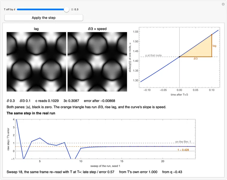
      

      Download ff-avg.wl

      Three frames, their average and the jump between q and it, over each frame's distance to the film as a share of q's, with the average above the nearest frame.
      What this draws, in Wolfram 15.0, 00:09
      # What obeys the rule survives the average; what ticks in unison cancels.

      What: a small disturbance that one third of a period and one slide multiply by , , sits in the three frames as times its size. The average keeps of it.

      Why: at the three arrows line up and it all stays. At a third of a turn round the unit circle they close into a triangle and it cancels. The film's own modes sit almost exactly at those angles.

      Try it: drag the orange dot, and watch the arrows close

      Where is. Black: the average cancels it. White: it all stays. Dots: the film's modes.

      The three frames' arrows, head to tail. Orange: the sum over , what the average keeps.

      the average keeps

      Frames in the average, :

      Where the factor comes from, and the test that it is real

      Write for simulate, for slide, and for the map, linearised at the film. commutes with exactly, so , and the line's three frames are , , . The average is

      and when ,

      And has its zeros at the two other cube roots of 1, , on the unit circle. With frames, has its zeros at the -th roots of 1 except 1. That is what the chips move.

      The measured test: the exact frame plus of the mode, one real run of the three frames with no free period, read in the mode's plane (find-film-modes.json, block m3_factor_is_real). The formula, then what the real program did:

      modeformulameasured
      unison1.1608119.81°0.0302710.030271
      time shift1.00000°1.0000001.000000
      slow0.52350°0.8184800.818480
      star imbalance0.96660°0.9887670.988767
      3-fold-breaking1.0153-120.07°0.0030140.003014

      The next card runs that test live, arrow by arrow.

      Why the film's modes sit near and , and when they would not

      This is the fact the method lives on. Of all 2592 modes, none is farther than 1.06° from or (find-film-modes.json, block m3e_bare_by_size). The reason shows at the rest state. Near rest a wave goes as , and because both chemicals diffuse at the same rate, every wave has the same (see why three waves). A third of a period turns any wave by . The slide turns it by a further or . So can only be or . That the film's modes stay within a degree of those angles at full amplitude is measured, not derived.

      So it depends on two things: the two chemicals diffusing alike, and being close to the rest state's clock. Change them and nothing lines up. At the settings of the true r33₁3₂ film of section 15, , the angle at the rest state is 146° for the uniform wave and 83° for the first shell, against 120.7° for every shell here. And that film's unison mode has 5.89 at 170.6°, nowhere near a zero: the average keeps 0.81 of it, and the free period makes that 4.77 a sweep (find-film-extra-E.json, block true_film_unison). That is why the program fails there.

      Where the comment oversimplifies

      "Cancels" needs near 1. The zeros are points on the circle. A mode at but well inside it is not cancelled, and as every angle gives , because the first frame keeps its weight. Across all 2592 modes, near :

      modesthe average keeps
      0.9 and up60.003 to 0.030
      0.5 to 0.980.043 to 0.073
      0.2 to 0.5220.108 to 0.188
      0.05 to 0.2260.207 to 0.247
      under 0.00115700.316 to 0.333

      Those fast modes are killed by the free period's , not by the average: both together.

      "What obeys the rule survives" is too narrow. Only obeys the rule: the time shift, and, before the first line removes them, the two translations. The slow mode does not obey it, and the average keeps 0.8185 of it anyway, since its arrows nearly line up. The average does not test the rule; it only cancels what is near a zero. What remains is decayed by the free period.

      "Ticks in unison" is a name. The unison mode is 60.7% spatial mean at the , 57.2% to 61.3% round the loop, and it holds other waves too (find-film-modes.json, block m3f_modes_round_the_loop). It is called that because a field with no pattern at all, every point ticking together, has at the rest state.

      Why three frames: measured, and not a law

      The rate one sweep can reach is the biggest factor among the modes the first line leaves, once the free period's is included; the chips show that number. At one free period (seeds 9001-9040, find-film-runs.json, block frames_grid):

      frames factor, predictedsweeps, measuredperiods simulated
      20.59744762.7
      30.42842643.3
      40.38982448.0
      60.32642053.3

      From three up, more frames take fewer sweeps and cost more simulated time, and two lets the unison through: three is the cheapest in periods at one free period. At two free periods the zeros at matter more: costs 40 periods, 75, 73, 48, since only 3 and 6 have them.

      It is this spectrum, not a law of a slide of order 3. With no free period is the cheapest, 69.8 periods against 71.3, because then nothing has made the unison grow: three frames are needed here because a free period lets it. And is no average: the program fails, 40 of 40 (the card above).

      Mathematica
      (* The factor (1 + mu + mu^2)/3: how much of a mode the average of three frames keeps. Left, the complex plane of mu, black where the factor is zero, white where it is 1 or more, with the film's real modes as dots. Drag the orange point: right, the arrows 1, mu, mu^2 head to tail, and in orange their sum over m. Evaluates in about 6 s on an M5: it finds the film, then measures the modes for real. *)
      
      n = 36; box = 40.;   (* a triangular mesh of n x n nodes, in a repeating box of this side *)
      a = 1.; b = 2.3;     (* the Brusselator's constants; both chemicals diffuse at rate 1 *)
      dt = 0.02;           (* the longest time step *)
      
      (* How fast the chemicals q = {u, v} are changing: diffusion plus reaction. *)
      laplacian[f_] := 2/(3 (box/n)^2) ListCorrelate[{{1, 1, 0}, {1, -6, 1}, {0, 1, 1}}, f, {2, 2}];
      rate[{u_, v_}] := {laplacian[u] + a - (b + 1) u + u^2 v, laplacian[v] + b u - u^2 v};
      
      (* Run time forward by t (fourth-order Runge-Kutta). *)
      simulate[q0_, t_] := Module[{q = q0, steps = Ceiling[t/dt], h, k1, k2, k3, k4},
         h = t/steps;
         Do[
          k1 = rate[q];
          k2 = rate[q + h/2 k1];
          k3 = rate[q + h/2 k2];
          k4 = rate[q + h k3];
          q += h/6 (k1 + 2 k2 + 2 k3 + k4),
          {steps}];
         q];
      
      (* Slide the picture by a third of the box. On the film this costs T/3 of time. *)
      slide[q_] := RotateLeft[q, {0, n/3, 2 n/3}];
      
      (* Turn the picture 120 degrees about the origin. On the film this costs no time. *)
      turn[q_] := Table[f[[Mod[x - y, n] + 1, Mod[-y, n] + 1]], {f, q}, {y, 0, n - 1}, {x, 0, n - 1}];
      
      (* One frame of the film, its period T, and the number of sweeps it took. *)
      findFilm[q0_, T0_ : 6.355, tol_ : 1*^-10] := Module[{q, T = T0, third, twoThirds, lag, speed},
         q = (q0 + turn[q0] + turn[turn[q0]])/3;    (* costs no time, so impose it once and it stays *)
         Do[
          q = simulate[q, T];                       (* one free period: what decays, decays *)
          third = simulate[q, T/3];
          twoThirds = simulate[third, T/3];
      
          lag = slide[third] - q;                   (* zero on the film *)
          If[RootMeanSquare[Flatten[lag]] < tol, Return[{q, T, sweep}, Module]];
      
          (* T is off by 3 x lag / speed. Move it gently, since at first it's all noise. *)
          speed = rate[q];
          T -= Clip[3 Total[lag speed, 3]/Total[speed speed, 3], {-0.1, 0.1}];
      
          (* What obeys the rule survives the average; what ticks in unison cancels. *)
          q = (q + slide[third] + slide[slide[twoThirds]])/3,
          {sweep, 399}];
         $Failed];
      
      (* Start from the rest state plus white noise, and find the film. *)
      rest = {ConstantArray[a, {n, n}], ConstantArray[b/a, {n, n}]};
      noise[s_, amp_ : 0.1] := (SeedRandom[s]; rest + RandomVariate[NormalDistribution[0, amp], {2, n, n}]);
      
      {fflQ, fflT, fflSweeps} = findFilm[noise[1]];
      
      (* The map M: a third of a period and a slide, linearised at the film. A mode is a field v with M v = mu v. *)
      fflM[v_] := (slide[simulate[fflQ + 0.001 v, fflT/3]] - slide[simulate[fflQ - 0.001 v, fflT/3]])/0.002;
      
      (* Arnoldi: the modes' mu from k products with M inside one set of fields, keeping those it has resolved, largest first. *)
      fflModes[inSet_, k_] := Module[{basis = {Normalize[Flatten[inSet[noise[2] - rest]]]}, h = ConstantArray[0., {k + 1, k}], w, c1, c2, vals, vecs},
         Do[
          w = Flatten[inSet[fflM[ArrayReshape[Last[basis], {2, n, n}]]]];
          c1 = basis.w; w -= c1.basis; c2 = basis.w; w -= c2.basis;    (* Gram-Schmidt, twice *)
          h[[;; j, j]] = c1 + c2; h[[j + 1, j]] = Norm[w];
          AppendTo[basis, w/Norm[w]],
          {j, k}];
         {vals, vecs} = Eigensystem[h[[;; k, ;; k]]];
         Pick[vals, Thread[Abs[h[[k + 1, k]] vecs[[All, k]]] < 0.001]]];
      
      (* The modes the first line leaves (fflSym), and those it removes. *)
      fflTurned[v_] := (v + turn[v] + turn[turn[v]])/3;
      fflSym = fflModes[fflTurned, 60];
      fflAll = Join[fflSym, fflModes[# - fflTurned[#] &, 60]];
      fflAt[pred_] := First[Select[fflSym, pred]];
      fflUnison = fflAt[Im[#] > 0 &];
      fflSlow = fflAt[Im[#] == 0 && Abs[#] < 0.999 &];
      fflFast = Last[Select[fflAll, Abs[Arg[#]/Degree - 120] < 3 &]];    (* the smallest resolved near +120 degrees *)
      
      (* What the average of m frames keeps of a mode, and the factor a whole sweep leaves of the slowest mode but the time shift. *)
      fflKeep[z_, m_] := (1 + 0 z + Total[Table[z^k, {k, m - 1}]])/m;
      fflSlowest[m_] := Max[Abs[fflKeep[#, m]] Abs[#]^3 & /@ Select[fflSym, Abs[# - 1] > 0.001 &]];
      
      (* Typed: median sweeps and periods simulated, 40 seeds at each m, measured in Python. With m = 1, no average, T walks to 0 on 40 of 40. *)
      fflMeasured = <|2 -> {47, 62.67}, 3 -> {26, 43.33}, 4 -> {24, 48}, 6 -> {20, 53.33}|>;
      
      fflShade[m_] := fflShade[m] = Raster[
          Clip[Abs[fflKeep[Table[x + I y, {y, -1.2975, 1.3, 0.005}, {x, -1.2975, 1.3, 0.005}], m]], {0, 1}]^0.62,
          {{-1.3, -1.3}, {1.3, 1.3}}];
      
      fflChain[z_, m_] := Module[{stops, sum, ext},
         stops = ReIm /@ Accumulate[Prepend[NestList[z # &, 1., m - 1], 0.]];
         sum = Last[stops]/m;
         ext = Max[1.25, 1.22 Max[Abs[stops]]];
         Graphics[{{GrayLevel[0.85], Line[{{-ext, 0}, {ext, 0}}], Line[{{0, -ext}, {0, ext}}]}, {Gray, Circle[]},
           {RGBColor[0.75, 0.35, 0], Thickness[0.014], Arrowheads[0.07], Arrow[{{0, 0}, sum}]},
           {RGBColor[0.19, 0.29, 0.78], Thick, Arrowheads[0.05], Arrow /@ Partition[stops, 2, 1]},
           {RGBColor[0.75, 0.35, 0], Text["sum / " <> ToString[m], sum, {-1.1, 1.8}]},
           Table[Text[Which[k == 0, "1", k == 1, "\[Mu]", True, Superscript["\[Mu]", k]], Mean[stops[[{k + 1, k + 2}]]] + 0.11 ext Normalize[Cross[stops[[k + 2]] - stops[[k + 1]]]]], {k, 0, m - 1}]},
          PlotRange -> {{-ext, ext}, {-ext, ext}}, PlotRangePadding -> None]];
      
      fflPicture[z_, m_] := Graphics[{fflShade[m],
          {GrayLevel[0.5, 0.6], Line[{{-1.3, 0}, {1.3, 0}}], Line[{{0, -1.3}, {0, 1.3}}]},
          {RGBColor[1, 0.69, 0], Dashed, Circle[]},
          {EdgeForm[RGBColor[0.118, 0.165, 0.51]], White, Disk[ReIm[#], 0.022] & /@ fflAll},
          Inset[fflChain[z, m], {2.8, 0}, Center, {2.6, 2.6}],
          Text["Black: the average cancels \[Mu]. White: it all stays. Dots: the film's modes.", {0, 1.42}],
          Text["The frames' arrows, head to tail. Orange: their sum over m.", {2.8, 1.42}]},
         PlotRange -> {{-1.3, 4.1}, {-1.3, 1.55}}, PlotRangePadding -> None, ImageSize -> 760, BaseStyle -> 10];
      
      fflSay[z_, m_] := Module[{keep = Abs[fflKeep[z, m]], deg = Arg[z]/Degree},
         Which[
          m == 1, "One frame: one arrow, nothing to cancel. With no average the program fails: T walks to 0 on 40 of 40 seeds.",
          m != 3, Row[{"With ", m, " frames the zeros stand every ", 360/m, " degrees round the circle, all but 1 itself; \[PlusMinus]120 degrees is ", If[m == 6, "among them.", "not."]}],
          keep < 0.05, "The arrows close: the frames hold it at three phases a third of a turn apart, and the average all but removes it.",
          keep > 0.75, "The arrows nearly line up: the frames agree about it, and the average keeps it.",
          Abs[z]^3 < 0.6 && Abs[Abs[deg] - 120] < 12, "The angle of a zero, but well inside the circle: the arrows shrink before they can close, and the factor tends to 1/3. This one needs the free period.",
          True, "The arrows partly close: the average keeps some of it."]];
      
      Manipulate[fflPicture[Complex @@ Clip[fflPoint, {-1.3, 1.3}], fflFrames],
       {{fflPoint, ReIm[fflUnison]}, Locator, Appearance -> Graphics[{RGBColor[1, 0.69, 0], Disk[]}, ImageSize -> 14]},
       {{fflFrames, 3, "Frames in the average, m"}, {1, 2, 3, 4, 6}, ControlType -> SetterBar},
       Row[{Button["Unison", fflPoint = ReIm[fflUnison]], Button["Slow", fflPoint = ReIm[fflSlow]], Button["Time shift", fflPoint = {1., 0.}], Button["Fast, at 120 degrees", fflPoint = ReIm[fflFast]]}],
       Dynamic[With[{z = Complex @@ Clip[fflPoint, {-1.3, 1.3}]}, Column[{
           Row[{"|\[Mu]|\.b3 = ", NumberForm[Abs[z]^3, {4, 3}], "     arg \[Mu] = ", NumberForm[Arg[z]/Degree, {4, 1}], " degrees     the average keeps ", NumberForm[Abs[fflKeep[z, fflFrames]], {4, 4}]}],
           fflSay[z, fflFrames],
           If[fflFrames == 1, "", Row[{"A sweep's slowest factor at these frames: ", NumberForm[fflSlowest[fflFrames], {4, 4}], ". Measured over 40 seeds: ", fflMeasured[fflFrames][[1]], " sweeps, ", fflMeasured[fflFrames][[2]], " periods simulated."}]]}]]],
       ControlPlacement -> Bottom, SaveDefinitions -> True]
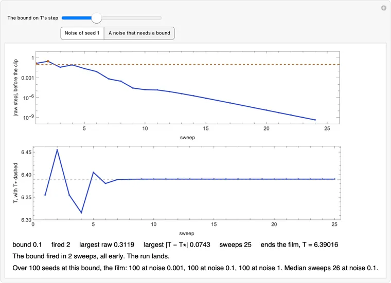
      

      Download ff-filter.wl

      The complex plane of mu shaded by the size of the factor, black at the two zeros on the unit circle, the film's real modes as dots, beside three arrows closing into a triangle.
      What this draws, in Wolfram 15.0, 00:06
      q = (q + slide(third) + slide(slide(two_thirds))) / 3

      What: the same arrows, for real. Start on the exact film plus a small push along one true mode, simulate, slide back. What the three frames hold beyond the film is three real fields; each is read as one arrow.

      Why: the factor on the last card is a formula about a linear map, and this line is real arithmetic. Here the three fields cancel on screen, or do not, and the arrows land on .

      Try it: pick a mode, and see whether its three frames cancel

      in q

      in slide(third)

      in slide(slide(two_thirds))

      in the average

      as arrows, measured; dashed:

      sum / 3, measured formula second arrow's error

      How a field becomes an arrow, and how close the arrows come

      The mode is , a complex eigenvector of with . A real push of size along it is . The real field goes to under , so is the field's coordinate in the mode's plane, and multiplies it by . To read an arrow: take the field and solve for the with , by least squares. A real mode has one coordinate, so its arrows lie along the axis.

      Nothing here is told : the dashed chain is drawn from the table, and the solid one from the run. The field's gap is second order in ; an arrow is that field divided by , so its error falls in proportion to , which is what the slider shows. For the unison mode (find-film-modes.json, block m8_arrows), the error in the second arrow is at , at , at . The page's eigenvectors are stored in 16 bits, which shows only near , where the error here is against in Python.

      What this shows and does not. It shows that the linear story is right for a small push on the film, which is where the run spends its late sweeps. Early in a run the field is far from the film, and the same reasoning has to start from the rest state instead; the slider's top end shows the arrows starting to bend.

      The whole sweep, and what each mode is

      The button runs the program's own sweep, free period and all, with held at . Its factor is , and at in Python (find-film-modes.json, block m3_factor_is_real), formula then measured: unison 0.035139, 0.035139; slow 0.428443, 0.428443; star imbalance 0.955697, 0.955697.

      Unison: 1.1608, the one mode of the symmetric fields that grows under plain simulation. Slow: the largest that decays with , of the fields the first line leaves, so the average barely touches it: it sets the pace, two cards on. Most of it, 53.4% to 70.9% round the loop, lies on the second star of waves (0,2), (2,-2), (-2,0) with their conjugates. Time shift: the frame a little later in time, which is still the film, so . It is what speed is, to . Star imbalance: the three waves' sizes changing with their sum fixed, 0.9666, ; it breaks the turn, so the first line removes it. Without that line it would set the pace, at 0.9557 a sweep. 3-fold-breaking: 1.0153, it grows, and at the average removes it anyway (factor 0.0030) even without the first line.

      Mathematica
      (* The arrows of the average, for real. Start on the film plus a small push along one true mode, really simulate, slide back: three real fields, read as arrows in the mode's plane, over the formula's dashed 1, mu, mu^2. Evaluates in about 7 s on an M5: it finds the film and measures the modes; each control then runs the simulation again. *)
      
      n = 36; box = 40.;   (* a triangular mesh of n x n nodes, in a repeating box of this side *)
      a = 1.; b = 2.3;     (* the Brusselator's constants; both chemicals diffuse at rate 1 *)
      dt = 0.02;           (* the longest time step *)
      
      (* How fast the chemicals q = {u, v} are changing: diffusion plus reaction. *)
      laplacian[f_] := 2/(3 (box/n)^2) ListCorrelate[{{1, 1, 0}, {1, -6, 1}, {0, 1, 1}}, f, {2, 2}];
      rate[{u_, v_}] := {laplacian[u] + a - (b + 1) u + u^2 v, laplacian[v] + b u - u^2 v};
      
      (* Run time forward by t (fourth-order Runge-Kutta). *)
      simulate[q0_, t_] := Module[{q = q0, steps = Ceiling[t/dt], h, k1, k2, k3, k4},
         h = t/steps;
         Do[
          k1 = rate[q];
          k2 = rate[q + h/2 k1];
          k3 = rate[q + h/2 k2];
          k4 = rate[q + h k3];
          q += h/6 (k1 + 2 k2 + 2 k3 + k4),
          {steps}];
         q];
      
      (* Slide the picture by a third of the box. On the film this costs T/3 of time. *)
      slide[q_] := RotateLeft[q, {0, n/3, 2 n/3}];
      
      (* Turn the picture 120 degrees about the origin. On the film this costs no time. *)
      turn[q_] := Table[f[[Mod[x - y, n] + 1, Mod[-y, n] + 1]], {f, q}, {y, 0, n - 1}, {x, 0, n - 1}];
      
      (* One frame of the film, its period T, and the number of sweeps it took. *)
      findFilm[q0_, T0_ : 6.355, tol_ : 1*^-10] := Module[{q, T = T0, third, twoThirds, lag, speed},
         q = (q0 + turn[q0] + turn[turn[q0]])/3;    (* costs no time, so impose it once and it stays *)
         Do[
          q = simulate[q, T];                       (* one free period: what decays, decays *)
          third = simulate[q, T/3];
          twoThirds = simulate[third, T/3];
      
          lag = slide[third] - q;                   (* zero on the film *)
          If[RootMeanSquare[Flatten[lag]] < tol, Return[{q, T, sweep}, Module]];
      
          (* T is off by 3 x lag / speed. Move it gently, since at first it's all noise. *)
          speed = rate[q];
          T -= Clip[3 Total[lag speed, 3]/Total[speed speed, 3], {-0.1, 0.1}];
      
          (* What obeys the rule survives the average; what ticks in unison cancels. *)
          q = (q + slide[third] + slide[slide[twoThirds]])/3,
          {sweep, 399}];
         $Failed];
      
      (* Start from the rest state plus white noise, and find the film. *)
      rest = {ConstantArray[a, {n, n}], ConstantArray[b/a, {n, n}]};
      noise[s_, amp_ : 0.1] := (SeedRandom[s]; rest + RandomVariate[NormalDistribution[0, amp], {2, n, n}]);
      
      {farQ, farT, farSweeps} = findFilm[noise[1], 6.355, 3*^-11];    (* a tighter tol, so the film's own error stays below the pushes *)
      
      (* The map M: a third of a period and a slide, linearised at the film. A mode is a field v with M v = mu v. *)
      farM[v_] := (slide[simulate[farQ + 0.001 v, farT/3]] - slide[simulate[farQ - 0.001 v, farT/3]])/0.002;
      
      (* Arnoldi: the modes {mu, v} from k products with M inside one set of fields, keeping those it has resolved, largest first. *)
      farModes[inSet_, k_] := Module[{basis = {Normalize[Flatten[inSet[noise[2] - rest]]]}, h = ConstantArray[0., {k + 1, k}], w, c1, c2, vals, vecs, good},
         Do[
          w = Flatten[inSet[farM[ArrayReshape[Last[basis], {2, n, n}]]]];
          c1 = basis.w; w -= c1.basis; c2 = basis.w; w -= c2.basis;    (* Gram-Schmidt, twice *)
          h[[;; j, j]] = c1 + c2; h[[j + 1, j]] = Norm[w];
          AppendTo[basis, w/Norm[w]],
          {j, k}];
         {vals, vecs} = Eigensystem[h[[;; k, ;; k]]];
         good = Thread[Abs[h[[k + 1, k]] vecs[[All, k]]] < 0.001];
         Transpose[{Pick[vals, good], Pick[vecs.Most[basis], good]}]];
      
      farTurned[v_] := (v + turn[v] + turn[turn[v]])/3;
      farSym = farModes[farTurned, 60];
      farBreak = farModes[# - farTurned[#] &, 60];
      
      (* One field per mode, scaled so that rms(Re v) is 1. A real mode has one coordinate; a complex one is turned so that Re v and Im v are at right angles. *)
      farScaled[{mu_, v_}] := Module[{w = If[Im[mu] == 0, Re[v], v Exp[-I Arg[v.v]/2]]}, {mu, ArrayReshape[w/RootMeanSquare[Re[w]], {2, n, n}]}];
      farPick[list_, pred_] := farScaled[First[Select[list, pred[First[#]] &]]];
      farMode = <|
         "Unison" -> farPick[farSym, Im[#] > 0 &],
         "Slow" -> farPick[farSym, Im[#] == 0 && Abs[#] < 0.999 &],
         "Time shift" -> {1., rate[farQ]/RootMeanSquare[Flatten[rate[farQ]]]},    (* a frame a little later in time: the film's own speed *)
         "Star imbalance" -> farPick[farBreak, Im[#] == 0 && Abs[#] < 0.999 &],
         "3-fold-breaking" -> farPick[farBreak, Im[#] > 0 &]|>;
      
      (* A field is read as an arrow z: the least-squares fit of field/eps = Re(z v). Each mode's mu is only used for the dashed chain. *)
      farReader[m_] := farReader[m] = PseudoInverse[Transpose[{Flatten[Re[farMode[m][[2]]]], -Flatten[Im[farMode[m][[2]]]]}], Tolerance -> 10^-6];
      farRead[m_, field_] := Complex @@ (farReader[m].Flatten[field]);
      
      (* The real run: the film plus a push, the two later frames, slid back. *)
      farFields[m_, eps_] := farFields[m, eps] = Module[{start = farQ + eps Re[farMode[m][[2]]], third, twoThirds},
          third = simulate[start, farT/3];
          twoThirds = simulate[third, farT/3];
          {start - farQ, slide[third] - farQ, slide[slide[twoThirds]] - farQ}/eps];
      
      (* And one whole sweep of the program, T held at the film's, with the same push: what it multiplies the push by. *)
      farSweep[m_, eps_] := Module[{q = simulate[farQ + eps Re[farMode[m][[2]]], farT], third, twoThirds},
         third = simulate[q, farT/3];
         twoThirds = simulate[third, farT/3];
         Abs[farRead[m, ((q + slide[third] + slide[slide[twoThirds]])/3 - farQ)/eps]]];
      
      (* Four points a mesh step, linear on the mesh's own triangles, as the page paints: a turned field then draws as the turned picture. *)
      meshTent = Table[Max[0., 1. - Max[Abs[i], Abs[j], Abs[i - j]]/4.], {j, -3, 3}, {i, -3, 3}];
      meshFine[f_] := ListCorrelate[meshTent, KroneckerProduct[f, Normal[SparseArray[{{1, 1} -> 1.}, {4, 4}]]], {4, 4}];
      
      (* The chemical u's deviation on the plane, black is zero, white is 2.6 times the push. *)
      farPane[u_, label_] := Labeled[Show[Quiet[
           ImageTransformation[Image[Clip[Abs[Reverse[meshFine[u]]]/2.6, {0, 1}]],
            {#[[1]] + #[[2]]/Sqrt[3.], 2 #[[2]]/Sqrt[3.]}/box + 0.5/(4 n) &, {300, 300},
            DataRange -> {{0, 1}, {0, 1}}, PlotRange -> {{-40., 40.}, {-40., 40.}},
            Padding -> "Periodic", Resampling -> "Linear"],
           RemoveAlphaChannel::imginv], ImageSize -> 150], label, Top];
      
      farChain[arrows_, formula_, sum_] := Module[{stops = ReIm /@ Accumulate[Prepend[arrows, 0.]], dashed = ReIm /@ Accumulate[Prepend[formula, 0.]], ext},
         ext = Max[1.25, 1.22 Max[Abs[Join[stops, dashed]]]];
         Graphics[{{GrayLevel[0.85], Line[{{-ext, 0}, {ext, 0}}], Line[{{0, -ext}, {0, ext}}]}, {Gray, Circle[]},
           {RGBColor[0.75, 0.35, 0], Thickness[0.016], Arrowheads[0.08], Arrow[{{0, 0}, ReIm[sum]}]},
           {Gray, Dashed, Line[dashed]},
           {RGBColor[0.19, 0.29, 0.78], Thick, Arrowheads[0.06], Arrow /@ Partition[stops, 2, 1]}},
          PlotRange -> {{-ext, ext}, {-ext, ext}}, ImageSize -> 180, PlotLabel -> "measured; dashed: 1, \[Mu], \[Mu]\.b2"]];
      
      farSay = <|"Unison" -> "The three fields differ, each a third of a turn on in the mode's plane. Added, they almost vanish: the average is nearly black, and the arrows close.",
         "Slow" -> "The same picture three times, a little fainter each time. Nothing cancels: the arrows lie in a line, and the average keeps most of it.",
         "Time shift" -> "The same picture three times. A frame a little later in time is still the film, so all of it stays.",
         "Star imbalance" -> "The same picture, nearly unchanged, so the average keeps nearly all of it. It breaks the 120 degree turn, so the first line removes it.",
         "3-fold-breaking" -> "This one grows, and it is cancelled all the same: its arrows close even more exactly than the unison's."|>;
      
      farView[m_, eps_, swept_] := Module[{fields = farFields[m, eps], mu = farMode[m][[1]], z, formula},
         z = farRead[m, #] & /@ fields;
         formula = {1., mu, mu^2};
         Style[Column[{
           Grid[{{farPane[fields[[1, 1]], "in q"], farPane[fields[[2, 1]], "in slide[third]"], farPane[fields[[3, 1]], "in slide[slide[twoThirds]]"],
              farPane[Mean[fields][[1]], "in the average"], farChain[z, formula, Mean[z]]}}, Spacings -> 0.3],
           Row[{"sum / 3, measured ", NumberForm[Abs[Mean[z]], {4, 4}], "     formula ", NumberForm[Abs[Mean[formula]], {4, 4}], "     second arrow's error ", ScientificForm[Abs[z[[2]] - mu], 2]}],
           Pane[farSay[m] <> If[eps >= 0.03, " At this size of push the arrows have left the formula: the response is no longer linear.", ""], 780],
           If[swept === {m, eps}, Row[{"One real sweep multiplied the push by ", NumberForm[farSweep[m, eps], {4, 4}], ". The formula, ", "\[Mu]\.b3 (1 + \[Mu] + \[Mu]\.b2)/3: ", NumberForm[Abs[mu^3 Mean[formula]], {4, 4}], "."}], ""]}, Spacings -> 0.7], FontFamily -> "Helvetica", 12]];
      
      Manipulate[farView[farWhich, farEps, farSwept],
       {{farWhich, "Unison", "Mode to push along"}, Keys[farMode], ControlType -> SetterBar},
       {{farEps, 0.001, "Size of the push"}, {0.00001, 0.0001, 0.001, 0.01, 0.03, 0.1, 0.3}, ControlType -> Slider, Appearance -> "Labeled"},
       Button["Run one real sweep", farSwept = {farWhich, farEps}, ImageSize -> Automatic],
       {{farSwept, None}, ControlType -> None},
       SaveDefinitions -> True]
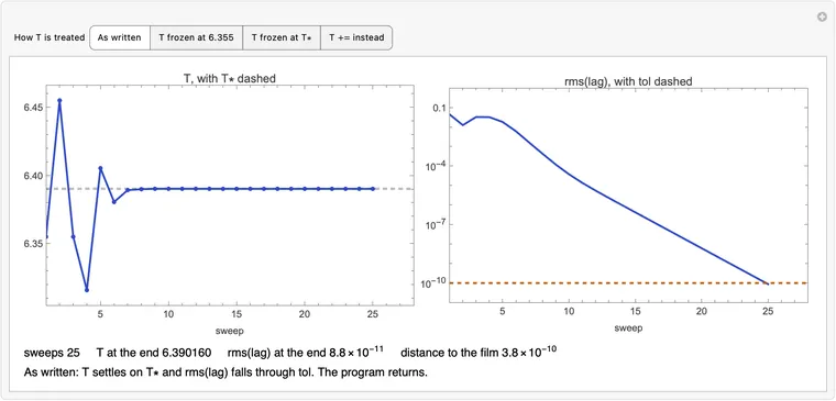
      

      Download ff-arrows.wl

      Three real deviation fields from a push along the unison mode, their nearly black average, and the arrows read from them closing over the formula's dashed triangle.
      What this draws, in Wolfram 15.0, 00:06
      q = (q + slide(third) + slide(slide(two_thirds))) / 3

      What: from noise, this line picks which waves grow. Within two sweeps three waves tower over the rest, at to each other: the film's pattern.

      Why: near the rest state every wave ticks at one clock, and is a third of its turn. The slide adds or , by wave. For one class the two cancel and the arrows line up; for the other two they close.

      Try it: scrub the sweeps, and tap a wave

      Measured: the size of each wave in the field, scaled to the largest. Centre: uniform.

      Predicted: what the step chosen below multiplies each wave by. Solid: it grows. Ring: it shrinks.

      Blue: the class whose arrows line up. Grey: the other two. Dashed orange: the film's three waves. Thick orange: the wave you tapped.

      the three waves the three opposite waves ratio

      The derivation, and the wave-by-wave test

      Near the rest state the equation is linear. Its Jacobian has eigenvalues with 0.15 and 0.9887. A wave feels the mesh's Laplacian as a number,

      Both chemicals diffuse at the same rate, so that number only shifts the growth: , and every wave keeps the same .

      The slide multiplies the wave by . So one third of a period and a slide multiply it by

      and a sweep multiplies it by

      Now at , to -0.0016° (that is why was the start). So for . Class 2 is on the filter's open point. The others sit near its zeros, and are stopped as far as allows.

      The test: rest state plus of one wave, one real sweep, read the wave before and after, on 19 waves. Worst relative error (find-film-modes.json, block m5_three_waves). And each piece alone, formula then measured (find-film-extra-E.json, block waves, worst relative error ):

      wavefree period alonethe average alonethe sweep
      uniform(0, 0)120°2.594, 2.5940.257, 0.2570.668, 0.668
      the star(1, 0)0°2.106, 2.1061.308, 1.3082.755, 2.755
      its opposite(-1, 0)-120°2.106, 2.1060.186, 0.1860.392, 0.392
      second star(-2, 0)0°1.134, 1.1341.043, 1.0431.183, 1.183

      Read the middle columns. By itself the free period favours the uniform wave, 2.59 a period against 2.11, and it cannot tell the star from its opposite: 20 of 20 runs of plain simulation end nearly uniform. The average turns that round. So the pattern is chosen here, not by the free period.

      The envelope: what the dots measure, and which three waves

      A real field holds every wave with its conjugate, so a plain Fourier transform of shows all six of the first shell at one size, and the selection cannot be seen. To see it, take the rest state's Jacobian, with its right eigenvector for and its left one, scaled so , and form the complex field . That keeps only the part of turning forward at . The dots are the sizes of its Fourier transform.

      The survivors for are . They add to , and with the mesh's inner product the cosine between any two is -0.5: three waves at . Read through the same field shows the negatives, , since that is the same field's conjugate. The turn sends , a 3-cycle on the three, so after the first line they are one number: their spread is at most through sweep 8, over 20 seeds.

      From noise, medians over 20 seeds: at sweep 0 the three are 0.0022 against 0.0023 for the others of that shell; top three by size on 1 of 20 seeds. At sweep 1, ratio 7.7, 19 of 20. At sweep 2, ratio 30.3, 20 of 20.

      Where "three waves" stops being the whole story

      Six indices grow, not three. For , of all 1296 indices exactly six have a factor over 1 at the rest state: the three at 2.755 and the second star at 1.183. That second star is class 2 as well, and its only just exceeds 1. The lattice here draws the 61 indices with shell up to 32. On the 24 with shell 38 or 42 the factor is at most 0.030, and everywhere else it is below 0.009.

      The rest is not zero on the film. As the three waves saturate, the ratio falls again: the others of their shell, the "cut" set, settle at 0.059 on the film against 0.234 for the star, at the published frame. That is not noise surviving. The noise's part falls away in two sweeps, and these are driven by the star through the reaction's nonlinearity: in the run the cut set grows as the star to the power 1.94 over sweeps 3 to 6. The scrubber shows the ratio peak at sweep 2 and come down.

      The linear story ends at saturation. is the rest state's, so on the film is a coordinate, not a mode's size. By seed 1's sweep 7 the three stop growing, at about 0.235: what the reaction allows, not what this line chose.

      It takes the turn too. A plane wave also passes this filter, since each of the three passes alone. Which is why, without the first line, the program mostly lands on one of them. The turn forces all three to one size. Slide and turn together make the star; the slide alone does not.

      Mathematica
      (* Why three waves. From noise, the size of each Fourier wave of the complex envelope, sweep by sweep, on the hexagonal lattice of wave indices; beside it, the factor predicted for each wave. Tap a wave for its three arrows. Evaluates in about 1 s on an M5: it really runs ten sweeps of the program; another noise costs a second more. *)
      
      n = 36; box = 40.;   (* a triangular mesh of n x n nodes, in a repeating box of this side *)
      a = 1.; b = 2.3;     (* the Brusselator's constants; both chemicals diffuse at rate 1 *)
      dt = 0.02;           (* the longest time step *)
      
      (* How fast the chemicals q = {u, v} are changing: diffusion plus reaction. *)
      laplacian[f_] := 2/(3 (box/n)^2) ListCorrelate[{{1, 1, 0}, {1, -6, 1}, {0, 1, 1}}, f, {2, 2}];
      rate[{u_, v_}] := {laplacian[u] + a - (b + 1) u + u^2 v, laplacian[v] + b u - u^2 v};
      
      (* Run time forward by t (fourth-order Runge-Kutta). *)
      simulate[q0_, t_] := Module[{q = q0, steps = Ceiling[t/dt], h, k1, k2, k3, k4},
         h = t/steps;
         Do[
          k1 = rate[q];
          k2 = rate[q + h/2 k1];
          k3 = rate[q + h/2 k2];
          k4 = rate[q + h k3];
          q += h/6 (k1 + 2 k2 + 2 k3 + k4),
          {steps}];
         q];
      
      (* Slide the picture by a third of the box. On the film this costs T/3 of time. *)
      slide[q_] := RotateLeft[q, {0, n/3, 2 n/3}];
      
      (* Turn the picture 120 degrees about the origin. On the film this costs no time. *)
      turn[q_] := Table[f[[Mod[x - y, n] + 1, Mod[-y, n] + 1]], {f, q}, {y, 0, n - 1}, {x, 0, n - 1}];
      
      (* Start from the rest state plus white noise, and find the film. *)
      rest = {ConstantArray[a, {n, n}], ConstantArray[b/a, {n, n}]};
      noise[s_, amp_ : 0.1] := (SeedRandom[s]; rest + RandomVariate[NormalDistribution[0, amp], {2, n, n}]);
      
      (* The rest state's clock. Near rest a field turns at sigma + i omega, and only the left eigenvector's part of it turns forward. *)
      ffoJacobian = {{b - 1, a^2}, {-b, -a^2}};
      {ffoGrow, ffoRight} = First[Select[Transpose[Eigensystem[ffoJacobian]], Im[First[#]] > 0 &]];
      ffoLeft = #/(#.ffoRight) &[Last[First[Select[Transpose[Eigensystem[Transpose[ffoJacobian]]], Im[First[#]] > 0 &]]]];
      ffoT0 = 6.355;
      
      (* The size of each wave (m, k), e^(2 Pi I (m x + k y)/n), in the envelope A = left . (q - rest). The wave's entry is at {k, m}, mod n. *)
      ffoEnvelope[q_] := Abs[Fourier[ffoLeft.(q - rest), FourierParameters -> {-1, -1}]];
      ffoSize[row_, {m_, k_}] := row[[Mod[k, n] + 1, Mod[m, n] + 1]];
      
      (* The real program from noise: the first line, then ten sweeps. Its stop test cannot fire so early. *)
      ffoRun[s_] := ffoRun[s] = Module[{q0 = noise[s], q, T = ffoT0, third, twoThirds, lag, speed, rows},
          q = (q0 + turn[q0] + turn[turn[q0]])/3;
          rows = {ffoEnvelope[q]};
          Do[
           q = simulate[q, T];
           third = simulate[q, T/3];
           twoThirds = simulate[third, T/3];
           lag = slide[third] - q;
           speed = rate[q];
           T -= Clip[3 Total[lag speed, 3]/Total[speed speed, 3], {-0.1, 0.1}];
           q = (q + slide[third] + slide[slide[twoThirds]])/3;
           AppendTo[rows, ffoEnvelope[q]],
           {10}];
          rows];
      ffoRun[1];
      
      (* The waves drawn, at their true place on the hexagonal lattice; the three that survive for +omega; their opposites. *)
      ffoShell[{m_, k_}] := m^2 + k^2 + (m + k)^2;
      ffoWaves = Select[Tuples[Range[-6, 6], 2], ffoShell[#] <= 32 &];
      ffoPlace[{m_, k_}] := {m, (m + 2 k)/Sqrt[3.]};
      ffoStar = {{1, 0}, {0, -1}, {-1, 1}};
      ffoCut = -ffoStar;
      
      (* Near rest a third of a period and a slide multiply a wave by lambda. Both chemicals diffuse alike, so the mesh's Laplacian only changes its growth. *)
      ffoLambda[{m_, k_}] := Exp[(ffoGrow + 2/(3 (box/n)^2) (2 Cos[2 Pi m/n] + 2 Cos[2 Pi k/n] + 2 Cos[2 Pi (m + k)/n] - 6)) ffoT0/3] Exp[2 Pi I (2 m + k)/3];
      ffoFactor["free", w_] := Abs[ffoLambda[w]]^3;                                    (* the free period: three thirds, slide undone *)
      ffoFactor["bare", w_] := Abs[1 + ffoLambda[w] + ffoLambda[w]^2]/3;              (* the average *)
      ffoFactor["both", w_] := ffoFactor["free", w] ffoFactor["bare", w];             (* the whole sweep *)
      ffoGrowing[which_] := Count[ffoWaves, w_ /; ffoFactor[which, w] > 1];
      
      (* A lattice: a dot's area is its value. Blue: the class of waves the slide leaves in step, 2 m + k = 2 mod 3. Dashed rings: the three. Orange ring: the wave tapped. *)
      ffoLattice[value_, top_, solid_, tapped_] := Graphics[{
          Table[With[{p = ffoPlace[w], r = Max[0.03, 0.56 Sqrt[Min[1, value[w]/top]]]},
            {If[Mod[2 w[[1]] + w[[2]], 3] == 2, RGBColor[0.19, 0.29, 0.78], Gray], If[solid[w], Disk[p, r], Circle[p, r]]}], {w, ffoWaves}],
          {RGBColor[1, 0.69, 0], Dashed, Circle[ffoPlace[#], 0.62] & /@ ffoStar},
          {RGBColor[0.75, 0.35, 0], Thick, Circle[ffoPlace[tapped], 0.72]}},
         PlotRange -> {{-5.1, 5.1}, {-5.1, 5.1}}, ImageSize -> 320];
      ffoNearest[pt_] := First[MinimalBy[ffoWaves, Norm[ffoPlace[#] - pt] &]];
      
      (* The tapped wave's arrows 1, lambda, lambda^2, head to tail, and in orange their sum over 3. *)
      ffoArrows[w_] := Module[{la = ffoLambda[w], stops, ext},
         stops = ReIm /@ Accumulate[{0, 1, la, la^2}];
         ext = Max[1.25, 1.22 Max[Abs[stops]]];
         Graphics[{{GrayLevel[0.85], Line[{{-ext, 0}, {ext, 0}}], Line[{{0, -ext}, {0, ext}}]}, {Gray, Circle[]},
           {RGBColor[0.75, 0.35, 0], Thickness[0.02], Arrowheads[0.1], Arrow[{{0, 0}, Last[stops]/3}]},
           {RGBColor[0.19, 0.29, 0.78], Thick, Arrowheads[0.07], Arrow /@ Partition[stops, 2, 1]}},
          PlotRange -> {{-ext, ext}, {-ext, ext}}, ImageSize -> 170]];
      
      ffoNumber[x_, places_] := ToString[NumberForm[x, {5, places}]];
      ffoView[s_, sweep_, which_, tapped_, onTap_] := Module[{row = ffoRun[s][[sweep + 1]], sizes, star, cut, top, grow = ffoGrowing[which], la = ffoLambda[tapped]},
         sizes[w_] := ffoSize[row, w];
         star = Mean[sizes /@ ffoStar]; cut = Mean[sizes /@ ffoCut];
         top = Max[sizes /@ ffoWaves];
         Style[Column[{
            Row[{Labeled[ClickPane[ffoLattice[sizes, top, True &, tapped], onTap[ffoNearest[#]] &], Pane["Measured: the size of each wave, scaled to the largest. Centre: uniform.", 320], Top],
              Labeled[ClickPane[ffoLattice[ffoFactor[which, #] &, Max[ffoFactor[which, #] & /@ ffoWaves], ffoFactor[which, #] > 1 &, tapped], onTap[ffoNearest[#]] &], Pane["Predicted: what the step multiplies each wave by. Solid: it grows. Ring: it shrinks.", 320], Top]}, " "],
            "Blue: the class whose arrows line up. Grey: the other two. Dashed orange: the film's three waves. Thick orange: the wave you tapped.",
            Row[{"the three waves ", NumberForm[star, {4, 4}], "     the three opposite waves ", NumberForm[cut, {4, 4}], "     ratio ", NumberForm[star/cut, {4, 1}]}],
            <|"free" -> Row[{"Plain simulation: ", grow, " waves grow, the uniform one fastest, and the three opposite waves just as fast as the star. Nothing is chosen."}],
              "bare" -> Row[{"The average alone: only the class whose arrows line up passes, and of it just ", grow, " waves grow."}],
              "both" -> Row[{"The whole sweep: ", grow, " waves of these ", Length[ffoWaves], " grow. Everything else shrinks, whatever the noise put there."}]|>[which],
            Row[{ffoArrows[tapped], Pane[StringJoin["Wave (", ToString[tapped[[1]]], ", ", ToString[tapped[[2]]], "): \[Lambda] = ", ffoNumber[Abs[la], 3], " at ", ToString[Round[Chop[Arg[la], 10^-9]/Degree]],
                 " degrees, what a third of a period and a slide multiply it by. The free period multiplies it by ", ffoNumber[ffoFactor["free", tapped], 2], ", the average by ", ffoNumber[ffoFactor["bare", tapped], 2], ", the sweep by ", ffoNumber[ffoFactor["both", tapped], 2], "."], 440]}, " "]}, Spacings -> 0.7], FontFamily -> "Helvetica", 12]];
      
      Manipulate[ffoView[ffoNoise, ffoSweep, ffoWhich, ffoTapped, (ffoTapped = #) &],
       {{ffoSweep, 2, "Sweep (0: after the first line)"}, 0, 10, 1, Appearance -> "Labeled"},
       {{ffoWhich, "both", "Which factor is predicted"}, {"free" -> "Free period", "bare" -> "The average", "both" -> "The sweep"}, ControlType -> SetterBar},
       {{ffoNoise, 1, "Noise"}, Range[6], ControlType -> SetterBar},
       {{ffoTapped, {1, 0}}, ControlType -> None},
       SynchronousUpdating -> False, SaveDefinitions -> True]
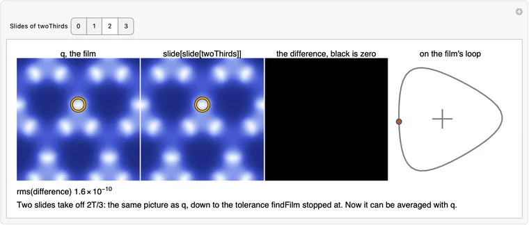
      

      Download ff-fourier.wl

      Two hexagonal lattices of Fourier indices: measured wave sizes at sweep 2, three dots at 120 degrees towering over the rest, beside the factor predicted for each wave.
      What this draws, in Wolfram 15.0, 00:01
      q = simulate(q, T)                          # one free period: what decays, decays
      q = (q + slide(third) + slide(slide(two_thirds))) / 3

      What: together the two lines multiply a mode by a sweep: from the free period, the rest from the average.

      Why: each line handles what the other cannot. The free period kills the fast modes and lets the unison grow; the average kills the unison and barely touches the slow ones. The largest factor left, 0.4284, sets the sweep count.

      Try it: switch a line off, then move the tolerance

      What a sweep leaves of each mode, on a log scale. An unnamed mode goes by its and angle. Orange: the largest, not counting the time shift.

      the largest each factor of 10 in tol

      Dashed: , with the largest factor above and read from this run's tail. Grey bars: the sweep at which each of 400 seeds stopped.

      sweeps: predicted, this run seed 1 median of 400 seeds

      The product, line by line, and the test

      A free period is three thirds with no slide. Since commutes with and , its derivative is , so an eigenvector of goes by . (At this it is only nearly so: simulate(q, T) takes 320 steps and three thirds 321. The real sweep's spectrum, by on the real 320 + 107 + 107 steps, agrees with the formula to on the slow mode and the star imbalance.) Then the average gives . The sweep's factor is the product. From the exact frame, one real sweep at , formula then measured (find-film-modes.json, block m3_factor_is_real):

      modefree, averagesweep, formulasweep, measured
      unison1.16080.03030.0351390.035139
      time shift1.00001.00001.0000001.000000
      slow0.52350.81850.4284430.428443

      The time shift's bar stays at 1 and has to: the film has no preferred instant. That does not stop the run, because the stop test reads lag, and on the time shift lag is zero.

      The step adds no factor of its own. On the pair the sweep's spectrum is this one plus a zero (the card on the 3): follows . With frozen at a run takes the same number of sweeps.

      Counting the sweeps: why the number is not 27

      With 0.4284, each factor of 10 costs 2.72 sweeps. It is tempting to say 27.2 and be done. But that assumes lag starts at size 1, and nothing sets that. The tail is , with read from the run: 0.052 to 3.47 over 120 seeds. Then , rounded up, is the count, on 119 of 120 seeds. So the count is explained by the factor and by one number from the run, and is what is not predicted: it holds what the first few nonlinear sweeps left behind.

      The line only fits late. Sweeps 8 to 12 fall 0.22 to 0.40 a sweep, faster than the slow mode, since faster modes still hold part of lag; only from about sweep 15 is it 0.40 to 0.43. And the slow mode here is the second star, not the amplitude of the three waves; that settles within seven sweeps.

      Measured, seeds 5001-5400: 400 of 400 reach the film, 21 to 30 sweeps, median 26. Below about the count stops being about the mode at all: lag reaches a floor, because the free period and the thirds take different step counts (the card on the stop test).

      What the other settings do to the race

      With no free period, the largest factor is the slow mode's bare 0.8185: 107 sweeps on seeds 1-40. They are cheaper sweeps, at 71.3 periods in all against 43.3 with one free period. With more, the slow mode falls faster but the unison rises: from the exact film its factor 1.1608 0.0303 crosses 1 at 24. From noise the limit comes sooner (the free-period count).

      Without the first line, the modes the turn had removed come back, and two kinds matter: the translations at 1, harmless, and the star imbalance at 0.9557, which sets the pace: a median of 363 sweeps on the star (the card on that line). No mode but the neutral ones is above that, so even on the whole mesh the film attracts the sweep, slowly.

      The bars are the modes the page holds: the largest of the turn-symmetric fields, by . Over the turn-symmetric modes the same formula puts only the time shift above the slow mode. Over all 2592 it adds the two translations and the star imbalance, and nothing else above 0.4284 (find-film-modes.json, block m3e_bare_by_size, with an independent dense check in m3d_dense_and_no_turn).

      Mathematica
      (* Both lines together: mu^3 from the free period, (1 + mu + mu^2)/3 from the average. Bars: what a sweep leaves of each mode, with the film's modes really measured. Below: rms(lag) of a real run against C f^sweep, with f the largest factor left: a tolerance becomes a sweep count, against the measured 400 seeds. Evaluates in about 4 s on an M5. *)
      
      n = 36; box = 40.;   (* a triangular mesh of n x n nodes, in a repeating box of this side *)
      a = 1.; b = 2.3;     (* the Brusselator's constants; both chemicals diffuse at rate 1 *)
      dt = 0.02;           (* the longest time step *)
      
      (* How fast the chemicals q = {u, v} are changing: diffusion plus reaction. *)
      laplacian[f_] := 2/(3 (box/n)^2) ListCorrelate[{{1, 1, 0}, {1, -6, 1}, {0, 1, 1}}, f, {2, 2}];
      rate[{u_, v_}] := {laplacian[u] + a - (b + 1) u + u^2 v, laplacian[v] + b u - u^2 v};
      
      (* Run time forward by t (fourth-order Runge-Kutta). *)
      simulate[q0_, t_] := Module[{q = q0, steps = Ceiling[t/dt], h, k1, k2, k3, k4},
         h = t/steps;
         Do[
          k1 = rate[q];
          k2 = rate[q + h/2 k1];
          k3 = rate[q + h/2 k2];
          k4 = rate[q + h k3];
          q += h/6 (k1 + 2 k2 + 2 k3 + k4),
          {steps}];
         q];
      
      (* Slide the picture by a third of the box. On the film this costs T/3 of time. *)
      slide[q_] := RotateLeft[q, {0, n/3, 2 n/3}];
      
      (* Turn the picture 120 degrees about the origin. On the film this costs no time. *)
      turn[q_] := Table[f[[Mod[x - y, n] + 1, Mod[-y, n] + 1]], {f, q}, {y, 0, n - 1}, {x, 0, n - 1}];
      
      (* Start from the rest state plus white noise, and find the film. *)
      rest = {ConstantArray[a, {n, n}], ConstantArray[b/a, {n, n}]};
      noise[s_, amp_ : 0.1] := (SeedRandom[s]; rest + RandomVariate[NormalDistribution[0, amp], {2, n, n}]);
      
      (* The program, keeping rms(lag). *)
      {fsfQ, fsfT, fsfLag} = Module[{q0 = noise[1], q, T = 6.355, third, twoThirds, lag, speed, lags = {}},
         q = (q0 + turn[q0] + turn[turn[q0]])/3;
         Do[
          q = simulate[q, T];
          third = simulate[q, T/3];
          twoThirds = simulate[third, T/3];
          lag = slide[third] - q;
          AppendTo[lags, RootMeanSquare[Flatten[lag]]];
          If[Last[lags] < 1*^-10, Break[]];
          speed = rate[q];
          T -= Clip[3 Total[lag speed, 3]/Total[speed speed, 3], {-0.1, 0.1}];
          q = (q + slide[third] + slide[slide[twoThirds]])/3,
          {399}];
         {q, T, lags}];
      
      (* The map M: a third of a period and a slide, linearised at the film. A mode is a field v with M v = mu v. *)
      fsfM[v_] := (slide[simulate[fsfQ + 0.001 v, fsfT/3]] - slide[simulate[fsfQ - 0.001 v, fsfT/3]])/0.002;
      
      (* Arnoldi: the modes' mu from k products with M among the fields the first line leaves, largest first. *)
      fsfTurned[v_] := (v + turn[v] + turn[turn[v]])/3;
      fsfModes[k_] := Module[{basis = {Normalize[Flatten[fsfTurned[noise[2] - rest]]]}, h = ConstantArray[0., {k + 1, k}], w, c1, c2},
         Do[
          w = Flatten[fsfTurned[fsfM[ArrayReshape[Last[basis], {2, n, n}]]]];
          c1 = basis.w; w -= c1.basis; c2 = basis.w; w -= c2.basis;    (* Gram-Schmidt, twice *)
          h[[;; j, j]] = c1 + c2; h[[j + 1, j]] = Norm[w];
          AppendTo[basis, w/Norm[w]],
          {j, k}];
         Eigenvalues[h[[;; k, ;; k]]]];
      
      (* The nine largest modes, one of each conjugate pair, each with what the free period, the average and both leave of it. *)
      fsfFactor["free", mu_] := Abs[mu]^3;
      fsfFactor["bare", mu_] := Abs[1 + mu + mu^2]/3;
      fsfFactor["both", mu_] := fsfFactor["free", mu] fsfFactor["bare", mu];
      fsfTop = Take[Select[fsfModes[60], Im[#] >= 0 &], 9];
      fsfName[mu_] := Which[Abs[mu - 1] < 0.001, "time shift", Im[mu] != 0 && mu == First[fsfTop], "unison", mu == First[Select[fsfTop, Im[#] == 0 && Abs[#] < 0.999 &]], "slow",
         True, ToString[NumberForm[Abs[mu]^3, {3, 2}]] <> If[Im[mu] != 0, " at 120", " at 0"]];
      fsfLargest[which_] := First[MaximalBy[Select[fsfTop, Abs[# - 1] > 0.001 &], fsfFactor[which, #] &]];
      
      fsfBars[which_] := Module[{x = Log10[Max[#, 0.01]] &, top = fsfLargest[which], list = Reverse[fsfTop]},
         Graphics[{
           Table[With[{mu = list[[i]], v = fsfFactor[which, list[[i]]]},
             {Which[mu == top, RGBColor[0.75, 0.35, 0], Abs[mu - 1] < 0.001, Gray, True, RGBColor[0.19, 0.29, 0.78]], Rectangle[{-2, i - 0.34}, {x[v], i + 0.34}],
              Black, Text[fsfName[mu], {-2.04, i}, {1, 0}], Text[NumberForm[v, {4, 3}], {x[v] + 0.03, i}, {-1, 0}]}], {i, Length[list]}],
           {Dashed, Line[{{0, 0.4}, {0, Length[list] + 0.6}}]},
           {Text[#, {Log10[#], 0.1}] & /@ {0.01, 0.1, 1}}},
          PlotRange -> {{-2.55, 0.65}, {-0.2, Length[list] + 0.7}}, AspectRatio -> 0.33, ImageSize -> 720]];
      
      (* Typed from the measured runs (Python). 400 fresh seeds: how many stopped at each sweep. Then for each tol: the median sweep over 400 seeds, Missing where none stop. With no free period: 107 sweeps, median of 40 seeds. *)
      fsfStops = <|21 -> 1, 22 -> 3, 23 -> 2, 24 -> 14, 25 -> 49, 26 -> 176, 27 -> 125, 28 -> 24, 29 -> 5, 30 -> 1|>;
      fsfMedian = <|1.*^-2 -> 7, 1.*^-3 -> 9, 1.*^-4 -> 11, 1.*^-5 -> 13, 1.*^-6 -> 15, 1.*^-7 -> 18, 1.*^-8 -> 21, 1.*^-9 -> 24, 1.*^-10 -> 26, 1.*^-11 -> 29, 1.*^-12 -> Missing[]|>;
      
      (* The line C f^sweep through the run's tail. C is what the first nonlinear sweeps left behind: it is read from the run, not predicted. *)
      fsfC[f_] := Last[fsfLag]/f^Length[fsfLag];
      fsfPredict[tol_, f_] := If[f < 1, Max[1, Ceiling[Log[tol/fsfC[fsfFactor["both", fsfLargest["both"]]]]/Log[f]]], Missing[]];
      fsfChart[which_, tol_] := Module[{f = fsfFactor[which, fsfLargest[which]], c},
         c = If[which === "both", fsfC[f], fsfC[fsfFactor["both", fsfLargest["both"]]]];
         ListLogPlot[{If[which === "both", fsfLag, {{1, 10.^3}}], Table[{s, c f^s}, {s, 32}], {{1, tol}, {32, tol}}},
          Joined -> {True, True, True}, PlotMarkers -> {Automatic, None, None}, PlotStyle -> {RGBColor[0.19, 0.29, 0.78], Directive[RGBColor[0.75, 0.35, 0], Dashed], Directive[Black, Dashed]}, PlotRange -> {{1, 32}, {1*^-12, 1}},
          AxesLabel -> {"sweep", None}, PlotLabel -> "rms(lag), a real run; orange: C f^sweep; black: tol; grey bars: the sweep at which each of 400 seeds stopped",
          Epilog -> {Gray, KeyValueMap[Rectangle[{#1 - 0.2, Log[1*^-12]}, {#1 + 0.2, Log[1*^-12] + #2/400 Log[10.^12] 0.4}] &, fsfStops]}, ImageSize -> 720, AspectRatio -> 0.3]];
      
      fsfTolSay[which_, tol_] := Which[
         which === "bare", "Measured with no free period: 107 sweeps, on 40 seeds.",
         which === "free", "No stop to predict: the factor is above 1.",
         tol >= 1*^-2, "Too loose: 148 of 400 seeds stop at sweep 2 or 3, on a field that has not grown.",
         tol >= 1*^-4, "Early on, the run sits above the line, so the line predicts too few sweeps: faster modes still hold part of the lag.",
         tol == 1*^-11, "370 of 400 seeds stop; the others meet the floor under rms(lag) and raise. The factor is no longer the limit.",
         tol < 1*^-11, "Below the floor: rms(lag) never gets there, and the program raises on every seed. The prediction is for a run with no floor.",
         True, "The line through the run's tail reaches the tolerance here; C is what the first sweeps leave behind."];
      
      fsfView[which_, tol_] := Module[{top = fsfLargest[which], f, hit},
         f = fsfFactor[which, top];
         hit = FirstPosition[fsfLag, x_ /; x < tol, {Missing[]}][[1]];
         Style[Column[{
            fsfBars[which],
            Row[{"the largest: ", fsfName[top], ", ", NumberForm[f, {5, 4}], "     each factor of 10 in tol: ", If[f < 1, Row[{NumberForm[Log[10]/Log[1/f], {3, 2}], " sweeps"}], "never"]}],
            <|"both" -> "Every bar short of 1 but the time shift, which cannot be anything else. The slowest is the slow mode.",
              "free" -> "A plain simulation. The fast modes go, but the unison mode is past 1: it grows, and with no average the runs end nearly uniform.",
              "bare" -> "The average alone. The unison is gone, but nothing presses on the modes with their arrows in line: it works, at about four times the sweeps."|>[which],
            fsfChart[which, tol],
            Row[{"sweeps: predicted, this run ", fsfPredict[tol, f] /. _Missing -> "none", "     this run ", If[which === "both", hit /. _Missing -> "past the end", "-"], "     median of 400 seeds ", If[which === "both", fsfMedian[tol] /. _Missing -> "none stop", "-"]}],
            fsfTolSay[which, tol]}, Spacings -> 0.7], FontFamily -> "Helvetica", 12]];
      
      Manipulate[fsfView[fsfWhich, fsfTol],
       {{fsfWhich, "both", "Which lines act"}, {"both" -> "Both lines", "free" -> "Free period only", "bare" -> "Average only"}, ControlType -> SetterBar},
       {{fsfTol, 1.*^-10, "tol"}, Keys[fsfMedian], ControlType -> Slider, Appearance -> "Labeled"},
       SaveDefinitions -> True]
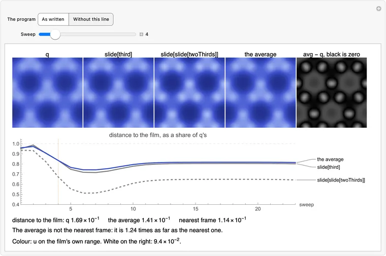
      

      Download ff-sweepfactor.wl

      Log-scale bars of what a sweep leaves of each measured mode, the slow mode longest at 0.428, over rms(lag) on the line C f^sweep with the histogram of 400 seeds at its foot.
      What this draws, in Wolfram 15.0, 00:04

      25. When it fails

      raise RuntimeError('no convergence')

      What: after 399 sweeps with lag never under tol, the program gives up.

      Why: so it cannot run for ever. At its own settings it never fires. Elsewhere it rarely means there is no film, and worse failures pass it by: a field with no film comes back with no error at all.

      Try it: move , then run the real program

      start steps at the it settles on: free period , three thirds

      Start : the rest state's clock at this , as the program's is at .

      Three different reasons it fires

      1. The film is found, and the arithmetic floor is over tol. This is the commonest. simulate(q, T) takes steps and three of simulate(q, T / 3) take . When those differ, the free period and the thirds are slightly different maps, and lag cannot fall below their difference. At that floor is under tol, to . Higher up it is not. From 2.62 to 3.30 in steps of 0.02, seeds 19001-19005: the program returns on all 5 at the 11 values where the counts agree, and raises on all 5 at the 24 where they differ. A comb, not a threshold. Run the free period as three thirds, one step length, and it lands at all six tried from 2.4 to 3.2, 120 of 120 runs (find-film-runs.json, blocks b_comb and b_why). The same comb is there in dt. The raise here says "no convergence" about a film it has in hand.

      2. Slowness at the threshold. With equal step counts, 2.06 to 2.07 raises on all 20 seeds at each: the first shell of waves starts to grow only at , so on each side of it the sweep's factor is near 1: 0.977 at 2.06, 0.9999 at 2.0656, 1.006 at 2.067. With the cap lifted it does end: rest at sweep 536 at ; a film at sweep 1425 at ; not within 2500 at .

      3. Really no film, for this program. At the settings of the true r33₁3₂ film of section 15 (), it raises on 24 of 24 and 24 of 24, from the rest state's clock and from the film's own. There the unison mode has 5.89 at 170.6°, far from the filter's zeros. The average keeps 0.81 of it, and the free period makes that 4.77 a sweep. Take out the free period and the method works: 20 of 24 land on that film's from the rest state's clock, 4 of 24 from the film's own, seeds 13001-13024 (find-film-runs.json, block true_film_k); section 15's count, one landing off, is a separate run of the bare average.

      The failures the raise does not catch

      These come back as a normal return, or as another error:

      • Rest, returned. Up to 2.055 a rest state comes back with no error, on all 20 seeds at each from 1.5. The is , but the waves the sweep can see only grow from . There is no film to find, and lag is small because the field is.
      • A tiny start, returned. At noise , lag is already under tol at sweep 1, on 100 of 100. The field is near rest, and is still 6.355.
      • near 0, returned. With a start , with no clip or a bound above 1, with too many free periods, or with a slide that is the identity, can walk down to about 0, where a field trivially matches itself. 20 of 20 from ; with no bound on the step, 8 of 300 fail, all but 1 of them this way.
      • A crash, not a raise. With of 0.59 and up, or noise from 5 up (1 of 40 at 5, 32 at 7, all 40 from 10), the numbers go to NaN and int(np.ceil(t / dt)) dies with ValueError: cannot convert float NaN to integer.

      So a caller should check and the spread of on what comes back. The raise alone will not catch these. On the published settings none of this arises: 400 of 400 reach the film, in at most 30 sweeps of the 399.

      Mathematica
      (* When the program gives up. A strip of what it did at each b, measured over many seeds and typed in, a comb and not a threshold; a slider for b; and the real program at that b, rms(lag) against sweep. Evaluating runs b = 2.68, a full raise of 399 sweeps, about 30 s on an M5; the Run button runs any other b. *)
      
      n = 36; box = 40.;   (* a triangular mesh of n x n nodes, in a repeating box of this side *)
      a = 1.; b = 2.3;     (* the Brusselator's constants; both chemicals diffuse at rate 1 *)
      dt = 0.02;           (* the longest time step *)
      
      (* How fast the chemicals q = {u, v} are changing: diffusion plus reaction. *)
      laplacian[f_] := 2/(3 (box/n)^2) ListCorrelate[{{1, 1, 0}, {1, -6, 1}, {0, 1, 1}}, f, {2, 2}];
      rate[{u_, v_}] := {laplacian[u] + a - (b + 1) u + u^2 v, laplacian[v] + b u - u^2 v};
      
      (* Run time forward by t (fourth-order Runge-Kutta). *)
      simulate[q0_, t_] := Module[{q = q0, steps = Ceiling[t/dt], h, k1, k2, k3, k4},
         h = t/steps;
         Do[
          k1 = rate[q];
          k2 = rate[q + h/2 k1];
          k3 = rate[q + h/2 k2];
          k4 = rate[q + h k3];
          q += h/6 (k1 + 2 k2 + 2 k3 + k4),
          {steps}];
         q];
      
      (* Slide the picture by a third of the box. On the film this costs T/3 of time. *)
      slide[q_] := RotateLeft[q, {0, n/3, 2 n/3}];
      
      (* Turn the picture 120 degrees about the origin. On the film this costs no time. *)
      turn[q_] := Table[f[[Mod[x - y, n] + 1, Mod[-y, n] + 1]], {f, q}, {y, 0, n - 1}, {x, 0, n - 1}];
      
      (* Start from the rest state plus white noise, and find the film. *)
      rest = {ConstantArray[a, {n, n}], ConstantArray[b/a, {n, n}]};
      noise[s_, amp_ : 0.1] := (SeedRandom[s]; rest + RandomVariate[NormalDistribution[0, amp], {2, n, n}]);
      
      (* findFilm at another b, Block changing b only for this run, keeping rms(lag) in frsLive as it goes. thirds runs the free period as three thirds, so all of it takes one step length. As in the Python, range(1, 400): 399 sweeps. *)
      frsLive = {};
      frsRun[bHere_, thirds_] := With[{q0 = noise[1] + {0., ConstantArray[(bHere - b)/a, {n, n}]}}, Block[{b = bHere}, Module[{q, T, third, twoThirds, lag, speed, status = "raised", sweeps = 399},
          T = frsStart[bHere];
          q = (q0 + turn[q0] + turn[turn[q0]])/3;
          frsLive = {};
          Do[
           q = If[thirds, Nest[simulate[#, T/3] &, q, 3], simulate[q, T]];
           third = simulate[q, T/3];
           twoThirds = simulate[third, T/3];
           lag = slide[third] - q;
           AppendTo[frsLive, RootMeanSquare[Flatten[lag]]];
           If[Last[frsLive] < 1*^-10, status = "returned"; sweeps = sweep; Break[]];
           speed = rate[q];
           T -= Clip[3 Total[lag speed, 3]/Total[speed speed, 3], {-0.1, 0.1}];
           q = (q + slide[third] + slide[slide[twoThirds]])/3,
           {sweep, 399}];
          <|"b" -> bHere, "thirds" -> thirds, "status" -> status, "sweeps" -> sweeps, "T" -> T, "spread" -> StandardDeviation[Flatten[q[[1]]]], "lags" -> frsLive|>]]];
      
      (* The rest state's clock, where T starts. At b = 4 the rest state has no clock left, and the runs started from 20. *)
      frsStart[bHere_] := If[bHere < 4, 2 Pi/Sqrt[a^2 - ((bHere - 1 - a^2)/2)^2], 20.];
      
      (* Typed from the measured runs (Python): {b, the T it ended on, what it did}. F a film, N no film and no error, R raised. Over 20 seeds at each of 2.06-2.07 and at grid values, 5 seeds from 2.62 to 3.3. *)
      frsTable = {
         {1.5, 5.8623, "N"}, {1.9, 6.2442, "N"}, {1.99, 6.2739, "N"}, {2.0, 6.2762, "N"}, {2.01, 6.2783, "N"}, {2.05, 6.2848, "N"}, {2.055, 6.2854, "N"},
         {2.06, 6.2860, "R"}, {2.0625, 6.2862, "R"}, {2.065, 6.2865, "R"}, {2.0656, 6.2866, "R"}, {2.067, 6.2869, "R"}, {2.07, 6.2881, "R"}, {2.075, 6.2898,
         "F"}, {2.08, 6.2916, "F"}, {2.09, 6.2952, "F"}, {2.1, 6.2989, "F"}, {2.2, 6.3401, "F"}, {2.3, 6.3902, "F"}, {2.4, 6.4501, "F"}, {2.5, 6.5199, "RF"},
         {2.6, 6.5992, "F"}, {2.62, 6.6161, "R"}, {2.64, 6.6333, "R"}, {2.66, 6.6509, "F"}, {2.68, 6.6687, "R"}, {2.7, 6.6869, "R"}, {2.72, 6.7053, "F"},
         {2.74, 6.7240, "R"}, {2.76, 6.7430, "R"}, {2.78, 6.7622, "F"}, {2.8, 6.7816, "R"}, {2.82, 6.8012, "R"}, {2.84, 6.8209, "F"}, {2.86, 6.8409, "R"},
         {2.88, 6.8610, "R"}, {2.9, 6.8812, "F"}, {2.92, 6.9014, "R"}, {2.94, 6.9218, "R"}, {2.96, 6.9422, "F"}, {2.98, 6.9626, "R"}, {3.0, 6.9829, "R"},
         {3.02, 7.0032, "F"}, {3.04, 7.0235, "R"}, {3.06, 7.0436, "R"}, {3.08, 7.0635, "F"}, {3.1, 7.0833, "R"}, {3.12, 7.1028, "R"}, {3.14, 7.1220, "F"},
         {3.16, 7.1410, "R"}, {3.18, 7.1596, "R"}, {3.2, 7.1778, "R"}, {3.22, 7.1955, "F"}, {3.24, 7.2129, "R"}, {3.26, 7.2297, "R"}, {3.28, 7.2460, "F"},
         {3.3, 7.2618, "R"}, {3.5, 7.3882, "R"}, {4.0, 17.9032, "R"}
         };
      frsStepCounts[t_] := {Ceiling[t/dt], 3 Ceiling[t/(3 dt)]};    (* the free period's RK4 steps, and three thirds' *)
      
      frsStrip[bHere_] := Module[{i = First[FirstPosition[frsTable[[All, 1]], bHere]], lanes = {"F" -> 3, "N" -> 2, "R" -> 1}, colour = <|"F" -> RGBColor[0.19, 0.29, 0.78], "N" -> Gray, "R" -> RGBColor[0.75, 0.35, 0]|>},
         Graphics[{
           {GrayLevel[0.85], Line[{{0, #}, {Length[frsTable] + 1, #}}] & /@ {1, 2, 3}},
           MapIndexed[Function[{row, at}, Table[{colour[l], PointSize[0.01], Point[{First[at], l /. lanes}]}, {l, Characters[Last[row]]}]], frsTable],
           {Black, Line[{{i, 0.5}, {i, 3.5}}]},
           Text["a film", {0, 3}, {1, 0}], Text["no film, no error", {0, 2}, {1, 0}], Text["raised", {0, 1}, {1, 0}],
           Text[If[# == 3., 3, #], {First[FirstPosition[frsTable[[All, 1]], #]], 0.2}] & /@ {1.5, 2.06, 2.3, 2.62, 3., 3.5}},
          PlotRange -> {{-9, Length[frsTable] + 1}, {0, 3.5}}, AspectRatio -> 0.16, ImageSize -> 720]];
      
      frsTells[row_, thirds_] := Module[{counts = frsStepCounts[row[[2]]], what = Last[row], bHere = First[row]},
         Which[
          thirds && StringContainsQ[what, "R"] && Unequal @@ counts, "Free period as three thirds: one step length, so no floor under lag. Press Run: from b = 2.4 to 3.2, 20 seeds at each, every run lands.",
          what === "N", "Returns on every seed, with no error: a rest state, no film. The raise never sees this.",
          what === "F", If[Equal @@ counts, "Lands on a film: the two step counts agree.", "Lands on a film: the two step counts differ, and the floor they make is still under tol."],
          bHere >= 3.9, "Raises: the field ends nearly uniform. Real eigenvalues at the rest state, so no clock to start from.",
          what === "R" && Equal @@ counts, "Raises with equal step counts: real slowness, at the threshold where the first waves start to grow.",
          what === "R", "Raises: the film is there, but the two step counts differ, and that sets a floor over tol.",
          True, "Raises on some seeds and not others: the floor straddles tol."]];
      
      frsChart[lags_] := ListLogPlot[{If[lags === {}, {{1, 1.*^20}}, lags], {{1, 1*^-10}, {Max[40, Length[lags] + 2], 1*^-10}}}, Joined -> True, PlotStyle -> {RGBColor[0.19, 0.29, 0.78], Directive[Black, Dashed]},
         PlotRange -> {{1, Max[40, Length[lags] + 2]}, {1*^-13, 10}}, AxesLabel -> {"sweep", None}, PlotLabel -> "rms(lag), with tol dashed", ImageSize -> 720, AspectRatio -> 0.26];
      
      frsResult[r_] := Row[If[r["status"] === "returned",
          {"Returned at sweep ", r["sweeps"], ", T = ", NumberForm[r["T"], {7, 6}], ", spread of u ", ScientificForm[r["spread"], 2], If[r["spread"] < 0.001, ": a rest state, and no error.", ": a film."]},
          {"RuntimeError at sweep 399. Least rms(lag): ", ScientificForm[Min[r["lags"]], 2], ", T = ", NumberForm[r["T"], {7, 6}], ", spread of u ", ScientificForm[r["spread"], 2], If[r["spread"] > 0.05, ": it has a film, and raises anyway.", "."]}]];
      
      frsShown = frsRun[2.68, False];
      frsNow[bHere_, thirds_, shown_] := Module[{row = First[Select[frsTable, First[#] == bHere &]], counts, fresh},
         counts = frsStepCounts[row[[2]]];
         fresh = shown["b"] == bHere && shown["thirds"] === thirds;
         Style[Column[{
            frsStrip[bHere],
            Row[{"start T, the rest state's clock at this b: ", NumberForm[frsStart[bHere], {5, 4}], "     steps at the T it settles on: free period ", If[thirds, counts[[2]], counts[[1]]], ", three thirds ", counts[[2]]}],
            frsTells[row, thirds],
            frsChart[If[fresh, shown["lags"], {}]],
            If[fresh, frsResult[shown], "Not run yet at this b. A full raise takes all 399 sweeps: about 30 s, and about 85 s at b = 4."]}, Spacings -> 0.7], FontFamily -> "Helvetica", 12]];
      
      Manipulate[frsNow[frsB, frsThirds, frsResultNow],
       {{frsB, 2.68, "b"}, frsTable[[All, 1]], ControlType -> Slider, Appearance -> "Labeled"},
       {{frsThirds, False, "How the free period is run"}, {False -> "As written", True -> "Free period as three thirds"}, ControlType -> SetterBar},
       Button["Run", frsResultNow = frsRun[frsB, frsThirds], Method -> "Queued", ImageSize -> Automatic],
       Dynamic[Row[{"The run so far: ", Length[frsLive], " sweeps, rms(lag) ", If[frsLive === {}, "-", ScientificForm[Last[frsLive], 2]]}]],
       {{frsResultNow, frsShown}, ControlType -> None},
       SaveDefinitions -> True]
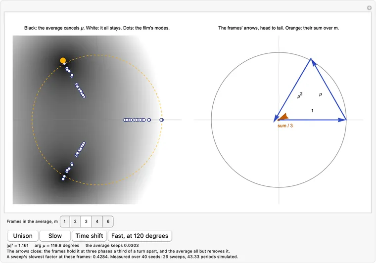
      

      Download ff-raise.wl

      A strip of what the program did at each measured b, a comb of landings and raises above 2.62, over a real run at b = 2.68 whose rms(lag) floors just over tol for 399 sweeps.
      What this draws, in Wolfram 15.0, 00:32

      26. Generators of the animation group

      The space-time symmetry group constructed in Parts 2 and 3 is the polar crystal group r33132 (built by adding time delays to wallpaper group 333), which the published film, built on three equal waves, completes to r32*3 (crystallographic space group R3m, No. 160) (section 15). In skewed hexagonal grid coordinates (i, j) ∈ [0, 1)2—where Cartesian position is x = L(i − ½j, (√3/2)j)—and period fraction τ = t/T ∈ [0, 1), here are the generators of the film find_film finds, in two forms: first by augmenting the original wallpaper-group generators of 333 with time shifts, and second as a minimal two-generator set.

      1. Wallpaper group 333 generators augmented with a time shift (Sections 9 & 10)

      Wallpaper group 333 can be presented either by the two side-pairing rotations of its rhombic fundamental domain (section 10) or by the three 120° rotations around the three inequivalent 3-fold centers A, B, C of its orbifold (section 9, linked by RARBRC ≡ 1 mod 1). Extending 333 to the polar crystal group r33132 simply attaches a fractional period shift τg = Δτ ∈ {0, +⅓, +⅔} to each spatial generator:

      333 generatorUnderlying 2D move on (i, j)Time shift ΔτAugmented space-time generator on (i, j, τ)
      Domain side ga (about (⅓, ⅓), anticlockwise)(⅔ − j, ⅓ + i − j)τa = +⅓(⅔ − j, ⅓ + i − j, τ + ⅓)
      Domain side gb (about (0, ⅓), anticlockwise)(⅓ − j, ⅔ + i − j)τb = +⅔(⅓ − j, ⅔ + i − j, τ + ⅔)
      Center A = (0, 0) (120° CW, axis 3)(−i + j, −i)0(−i + j, −i, τ)
      Center B = (⅔, 0) (120° CW, cost ⅔)(4/3 − i + j, ⅔ − i)+⅔(4/3 − i + j, ⅔ − i, τ + ⅔)
      Center C = (⅓, 0) (120° CW, cost ⅓)(⅔ − i + j, ⅓ − i)+⅓(⅔ − i + j, ⅓ − i, τ + ⅓)

      Because the product of the three clockwise turns around A, B, C is the identity mod 1, their time shifts must sum to an integer: 0 + ⅔ + ⅓ = 1 ≡ 0 (mod 1). Swapping the two shifts gives the same group in its other setting, not a new hand: a 180° turn about A does it. That is section 9's formula film, the program's waves turned 180° (on them, the same as reversing time), where the clockwise turn about B costs ⅓, about C ⅔, and the slide is (i + ⅓, j + ⅔, τ + ⅓).

      2. Minimal set of generators: point turn + space-time glide (Sections 15, 19 & 24)

      Composing gb ∘ ga−1 cancels the rotation and isolates a pure space-time translation, mod 1 the rhombus's long diagonal run backwards. This yields the minimal generating set of just two generators (implemented directly as turn and slide in Part 3, whose slide undoes the move in the table, shifting a picture by (⅓, ⅔) ≡ −(⅔, ⅓)), plus the emergent mirror m• (in 3D cube coordinates on (R / 2πZ)3, here X = 2π(i + τ), Y = 2π(j − i + τ), Z = 2π(τ − j); sections 9 and 15):

      GeneratorAction on (i, j, τ) mod 13D cube action on (X, Y, Z)Time shift ΔτOrder mod Z3
      turn (r)(−j, i − j, τ)(Z, X, Y) — cyclic permutation03
      slide (s)(i + ⅔, j + ⅓, τ + ⅓)(X + 2π, Y, Z) — 1-period edge shift+⅓3
      mirror (m•, carried by the three waves)(−j, −i, τ)(Z, Y, X) — swap two cube axes02

      Why two generators suffice (no separate y-shift or mirror needed): Modulo the periodic torus lattice Z3 of full grid wraps (i + m, j + n, τ + k) for (m, n, k) ∈ Z3, turn (r) and slide (s) commute: rotating the shift vector (⅔, ⅓) by 120° gives (−⅓, ⅓) ≡ (⅔, ⅓) (mod 1). Thus r and s alone generate all nine cosets rasb for a, b ∈ {0, 1, 2} of r33132 / Z3 (section 24), and conjugating slide by turn in the unrolled plane generates the second spatial lattice direction automatically. The film's three equal waves at 120° are automatically invariant under mirror (i, j, τ) ↦ (−j, −i, τ) (section 15); omitting mirror leaves room for chiral r33132 films, at other settings with Du ≠ Dv: the bare average finds one, and the program of section 16, with its free period, does not (section 15).